R Tutorial - An Introduction For Beginners

R Tutorial – An Introduction for Beginners

This tutorial is an introduction to the statistical programming language R and covers the basic syntax: variables and data types, data structures (vectors, matrices, data frames), control flow, functions, data visualization and the most important packages / libraries. We use RStudio and RStudio Cloud as an integrated, user-friendly development environment for R. A brief motivation is followed by the description on how to use the development environment RStudio, then a walk through R language, starting from the first print-commands to the more sophisticated data manipulations and visualizations. All features of the syntax are shown using example codes.

Motivation

R is a programming language and development environment for statistical calculations and graphics, developed in 1992 by statisticians Ross Ihaka and Robert Gentleman at the University of Auckland. R is the modern implementation of the statistical language S, which goes back as far as 1975.

R is used as standard language for statistical problems in teaching, science and business. Free R packages expand R's field of application to include many specialist areas. A thourough documentation and many forums dedicated to the use of R enable to easily grasp and use the functionality. Since the source code is public, R offers the possibility of quickly developing new packages and making them available. While R is not targeted for performance or real-time scenarios, it is great for statistics and data visualization.

RStudio is the free integrated development environment for the programming language R. While R was used in the beginning mostly as console program in interactive mode, today it allows to create projects with multiple script files and graphical user interfaces. The functionality offered by RStudio is similar to that offered by Spyder IDE for Python. RStudio Cloud is the cloud-based version of RStudio and requires no installation.

Overview

The tutorial is structured in ten sections that explain usage of the RStudio Development Environment and the most important R commands, data structures, plotting functionality and packages.

Environments: RStudio and RStudio Cloud

In order to work with R and RStudio, an R version must be installed from the R project website or from The Comprehensive R Archive Network: cran.r-project.org. Next, RStudio should be downloaded and installed from rstudio.com. The current version of R can be found out in the RStudio console using the command R.version, which displays information such as R version 4.0.5 (2021-03-31) and the nickname, "Shake and Throw".

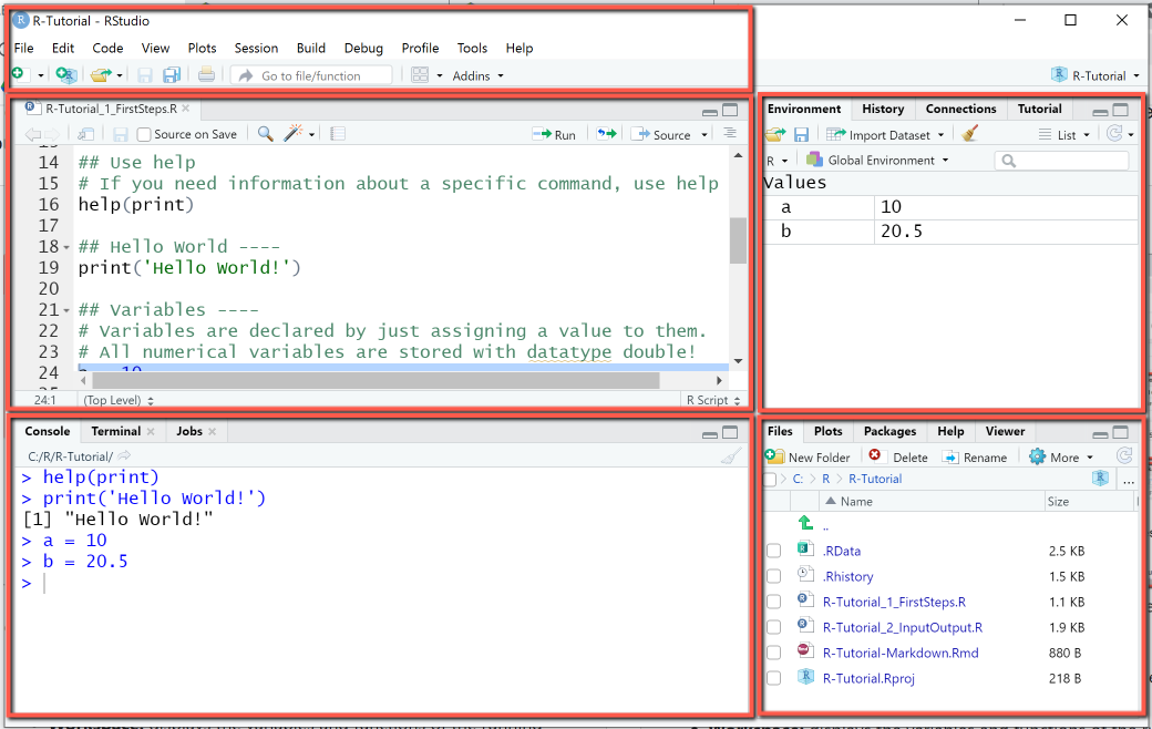
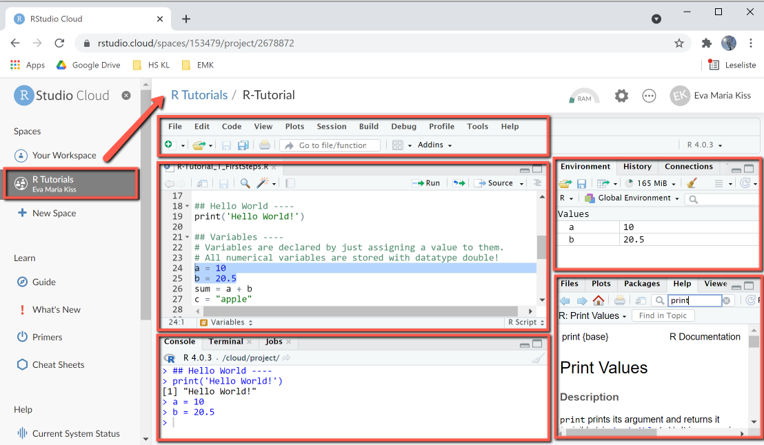
RStudio's default user interface is organized in four configurable panels, that are used for developing and running scripts. The configuration can be done using View > Panes > Pane Layout Menu, it is mainly restricted to selecting which views to display in which panel. The user interface of RStudio Cloud is very similar, except that it displays a sidebar on the left containing your workspaces and a breadcrumb navigation displaying the current project.

Menu bar: Basic functionality of the IDE is grouped in the menus File (creating files), Edit (undo, redo, search), Code (editing and running code), View, Plots, Session, Build.
Editor (top-left): displays the contents of the script files. The actual programming is done in the editor.
Console (bottom-left): shows the executed code and its output
Environment / History / Connections (top-right): Environment displays the variables and functions of current R Session, History the command history, so that you can easily recall previous commands, Connections are needed for example to connect to the cloud.
Files / Plots / Packages / Help : This panel groups a number of utility tabs needed for organizing files (where you save your data, scripts and projects), packages (here you check for installed packages and search for available packages), as well as plots and help.

RStudio Environment

RStudio Cloud

R execution modes

R code can be created and executed in different ways, it depends on the application which mode is best:

Interactive mode:
R can be used in interactive mode, by entering commands directly in the console and pressing the Enter key. Output is also shown in the console. Previous commands can be recalled with the up / down arrow keys or viewed in the history (tab next to Environment). Interactive mode is useful for tutorials and for testing small program parts.
R script:
Larger R programs are collections of R scripts (extension: .R) stored in a common folder that is used as the working directory. The current working directory is displayed with the getwd () (get working directory) command and can be set to any folder with setwd ("path").
R Markdown:
R Markdown is a special type of script with extended documentation features.

Create and run R scripts

An R script is a text file with the extension .R, that contains the statements and comments of the program. R script names may contain only letters, numbers and the characters dot (.) and subscript (_). The name may begin with a letter or a period, taking care that no number follows the leading period, and avoiding R keywords as they are not permitted as script names. Valid names are for example myscript1.R, myscript2.R, myfun1.R, myfun2.R.

Create R scripts:
R scripts are created using File > New File > R Script menu or the keyboard shortcut CTRL + Shift + N. A symbol (green plus symbol) for creating new scripts is also available in the menu bar.

Run R scripts:
R scripts are executed using the Code menu and its Run instructions, or the corresponding Run instructions in the Editor menu (Run, Source without Echo, Source with Echo). Run executes the line on which the cursor is located or the lines that have been marked.

1. First Lines in R

Top

R scripts contain statements (also: instructions) and comments. R statements are executable instructions: expressions, variable assignments, function calls. R statements are separated by newline, or, if multiple statements are placed on the same line, by semicolon.

Important: R is case sensitive, ie print(x) is not the same as Print(x).

Comments in R start with a "#"-symbol followed by text. Comments are used for documentation purpose, they make lines of code easier to understand and are not executed by the system. Everything in the line after a # symbol is marked as a comment and colored green by the syntax highlighter.

Lines of code can be entered directly in the console or saved in an R script and executed using the Run- and Source-menus. The Run- and Source- menus in RStudio offer different ways to execute a script:

Run executes the line on which the cursor is located or the lines that have been marked. If the script has no sections, the entire script is executed. If the script is structured in sections, pressing Run repeatedly will execute section after section. All comments, code lines and output are sent directly to the console and displayed there.
Source without echo: will source the entire source code of the script file to a temporary folder and then execute it. The console will display only the output of the script.
Source with echo: will source the entire source code of the script file to a temporary folder and then execute it. Comments, code lines and output are displayed on the console

Before starting to explore the R language, it is useful to learn some commands that are needed frequently for help or to keep a clean and organized workspace and console.

The console is cleared using the Edit > Clear console menu, or the shortcut CTRL + L. When writing larger scripts and running them in test cycles, it is often useful to include this as command at the beginning of the script. This is done with cat("\014") and will clear the console (instructions and output). Useful when you want to start over with a clean slate.
rm() – Clears environment variables. You can delete single variables - for example, rm(a) deletes the variable a, or all variables: rm(list = ls()) deletes all variables in the environment. Useful when you run multiple scripts that use the same variable names.
help – If you type help followed by the name of a command or function in parantheses, the corresponding help page is displayed. For example help(print) displays the help for the print function. The same effect is obtained by typing ?print.

Example: Find out what a command does

This example shows how to use help to find out information about the print-command.

R Code: Find out what a command does

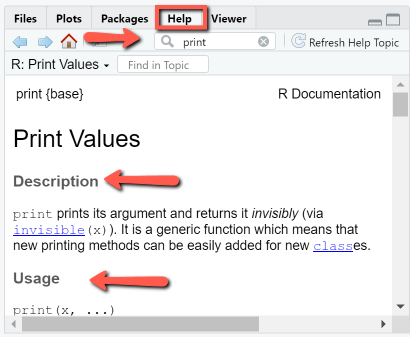
Using help and ?

When typing "help(print)" or "?print" in the console, the R documentation for the print command is shown in the bottom-right panel, as depicted. This panel can also be used directly. The R documentation page contains the description of the function, usage, arguments, details and examples.

> help(print)
> 
> ?print
>

Output

RStudio Console Panel after executing "Run"

Hello World-Programm in R

A Hello-World-program is the smallest runnable program in a programming language and prints the text "Hello World" to default output (here: the console). We do it first in interactive mode and then in an R script.

Example: Hello World in Interactive mode

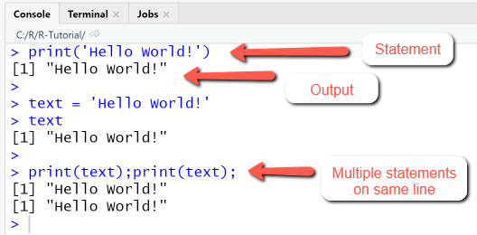
In this example we print the text "Hello World" to the console in three different ways: (1) by using the function print to display the string, (2) by declaring a variable "text" that stores the string + output its content to the console by just typing its name, and (3) by printing the content of "text" twice.

In interactive mode, statements are entered next to the the command prompt (indicated by >) in the console and executed by pressing ENTER. Pressing ENTER without any statement will start a new console line.

R Code

Using interactive mode and the console

First, type the statement

print('Hello World!')

in the console and press ENTER. Observe that the text is printed to the console, in black, with a line number.

Next, type the statement

text = 'Hello World!'

in the console and then press ENTER. No output is generated yet, but the variable appears in the workspace. At the next command prompt, type

text

and again press ENTER. As shown in the picture, the content of the variable (here: Hello World!) is shown as output in the console.
Last, type print(text) twice on a line, and separate the print-statements with a semicolon.

print(text);print(text)

Output

RStudio Console Panel

The difference between statement and output is recognizable from the command prompt and the coloring: statements are blue, output is black.

Usually a console line contains a single statement; if multiple statements are placed on the same line, they must be separated with a semicolon.

Example: "Hello World" in Script mode

In script mode, we first create a new script with the name "hello_world.R", then type the R statements below in the script file and save it, and finally execute the script using the Run-menu, which prints the script and the output to the console.

R Code

Using script files to store larger programs

The code starts in line 1 with a comment (indicated by "#"-symbol), that states the name of the script file. Note that the following lines are also commented. In line 4 we create a new variable "text" and assign it the value 'Hello world'. In line 5 we print the string 'Hello World' using disp().

# R-Tutorial: Hello World-Script
# Section 1 ----
# Output string using print
print("Hello World!")

# Section 2 ----
# Declare a variable and output its content
text ="Hello World!"
text

# Section 3 ----
# Two print-statements on the same line
print(text);print(text)

Output

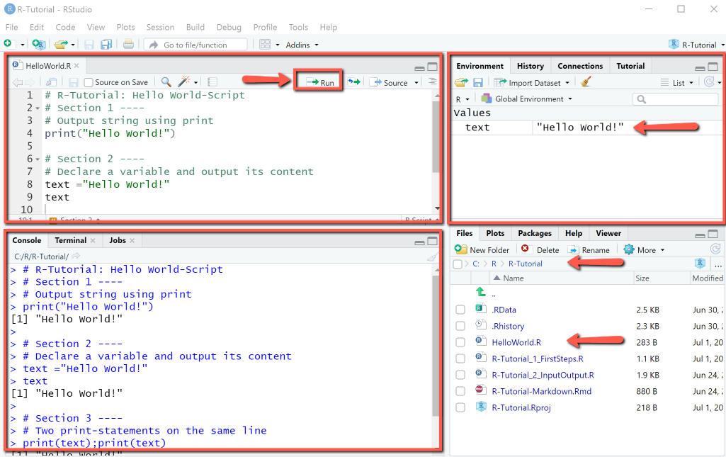
RStudio Integrated Development Environment

The RStudio IDE after creating, editing, saving and running the script hello_world.R with "Run" looks as shown. Top-left: the source code contains section breaks. Bottom-left: The console displays the source code and the output.

Comments in R

Comments in R start with a "#"-symbol followed by text. Comments are used for documentation purpose, they are not executed by the system.

A special type of comment is the section comment. Sections structure a script into regions, that can be executed separately using the Code > Run Region menu. The section comment consists of a "#"-symbol, followed by text and then at least four of the symbols "----". Sections can also be created using the Code > Insert section menu, but this can done more efficiently using the section comment.

## Section 1 ----
# Comment 1: This is the first comment for section 1. 
text = "Let's start simple" # Here we assign a value to the variable named text 
## Section 2 ----
# Comment 2: This is the first comment for section 2. 
a = 10 # Here we assign a value to variable a 
b = 20 # Here we assign a value to variable b

2. Variables and data types

Top

Variables are named storage locations to which values of different data types (numeric, integer, logical, character, string) and expressions can be assigned. R variables are declared by simply assigning a value to them, as in the next example. Here we consider only simple variables, vectors and matrices will be discussed in later sections.

2-1 Assignments

Top

An assignment is made using the assignment operator <- or alternatively the = operator. The <- and = operators have a different operator precedence, which is good to know when mixing them in the same expression. The assignment operator <- always points to the object receiving the value of the expression, this is an advantage, because it makes it unambiguous. Throughout this tutorial we will use the = operator, since this is more common in other programming languages.

Example: Variables

The example shows how to declare variables (numerical and strings) by assigning values and how to perform operations on variables.

Line 1-10: Declare two variables a, b by assigning values to them. The assignment for variable a is done using the = operator, the assignment for variable b using the <- operator. Add the two variables (actually, their values) and store the result in the variable sum.
Line 12-16: Declare two string variables s1, s2 and concatenate them using paste().

R Code: Variables

Declare variables by assignment

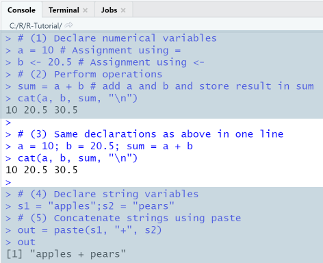
# (1) Declare numerical variables
a = 10 # Assignment using =
b <- 20.5 # Assignment using <-
# (2) Perform operations 
sum = a + b # add a and b and store result in sum
cat(a, b, sum, "\n")

# (3) Same declarations as above in one line
a = 10; b = 20.5; sum = a + b
cat(a, b, sum, "\n")

# (4) Declare string variables
s1 = "apples";s2 = "pears"  
# (5) Concatenate strings using paste
out = paste(s1, "+", s2)
out

Output

RStudio Console Panel after executing "Run"

When executing the script using the Run-menu item, output in console is as shown. Note that Run menu item will display the entire script in the console, including comments and code.

2-2 Data types

Top

The data type (numeric, integer, logical, string, etc.) of a variable is determined automatically by R. The basic data types in R are: Numeric, Integer, Complex, Logical, Character. The default data type for numbers in R is Numeric, that is, decimal values, even integer values are stored as Numeric.

In order to create variables of a specific data type, the R conversion functions as.integer, as.numeric, as.character etc. are used. In order to test for the data type of a variable, the functions is.integer, is.numeric, is.character etc. are used.

x = as.integer(10) # creates an integer
y = as.numeric(10) # creates a numeric
is.integer(x) # is x an integer?
is.numeric(y) # is y a numeric?

2-3 Find out type and structure of objects

Top

R provides utility functions for obtaining type and structure of variables and objects. These include the functions class, which displays the class of an object, typeof, which displays the data type of a variable, and str, which displays the internal structure of an R object. Another important utility function is summary, which displays the summary of statistical properties of R data structures (vectors, matrices, data frames).

These functions are often used for diagnostics, for example, when the result of an operation is not as expected or we do not know if a function has returned the correct result. Knowing the class of an object or data type of a variable is important, since these determine the set of operations that you can perform with objects.

Example: Find out type and structure of objects

This example shows how find out the class and data type of R objects and variables.

R Code

Using class, typeof, str and summary

We first declare a variable x and display its class and data type, then a vector y and display its internal structure and summary of its statistical properties.

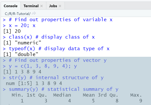
# Find out properties of variable x
x = 20; x
class(x) # display class of x
typeof(x) # display data type of x
# Find out properties of vector y
y = c(1, 3, 8, 9, 4); y
str(y) # internal structure of y
summary(y) # statistical summary of y

Output

When executing the script using the Run-menu item, output in console is as shown.

3. Output- and Input-Commands

Top

Data stored in variables can either be viewed in the environment or displayed in the console. While the environment shows the raw variable values, the console can be used for formatted output.

Output to console

There are multiple ways to output object values to console: by typing the variable name in a new line, or by using one of the functions print, cat, sprintf or message. Typing the variable name in a new line or using print are the most common ways and frequently used, but they both display a line number before the output, which is not always a desired effect. In this case, it is preferable to use the cat-function.

Simply type the name of a variable, either in a new line, or in the same line with semicolon as separator. The content of the variable then is displayed in the console and a line number is used, e.g. [1], [2].
Use print()-function. This function takes as argument a variable / vector / matrix and displays it, while also prepending a line number.
Use cat()-function. This function takes as argument a variable / vector / matrix and displays it without prepending a line number.
Use sprintf()-function. This function builds a formatted output by using placeholders for the variables to be inserted, in the same way as the known functions printf and fprintf from C language. In our example, the value of variable a will be inserted in the place indicated by the first "%d", the value of variable b will be inserted in the place indicated by the second "%d" etc.

Example: Output to console

In this example we calculate the sum of two variables and display output on console in four different ways.

R Code: Output to console

Using print, cat, sprintf

Line 3-6: Declare variable a and display its value by typing its name. Same for b. Then calculate sum of a and b. Display values of a, b and sum by typing the variable names in a new line, separated by comma.
Line 8: Create a vector using the statement c(a, b) and display it using print.
Line 9: Display value of sum using print. Note that print will display any object, be it variable, vector or matrix.
Line 11-12: Display a, b, and sum using cat. Line break ("\n") must be appended explicitly.
Line 13-14: Output with sprintf works using a formatting string, as in the well-known C-functions.

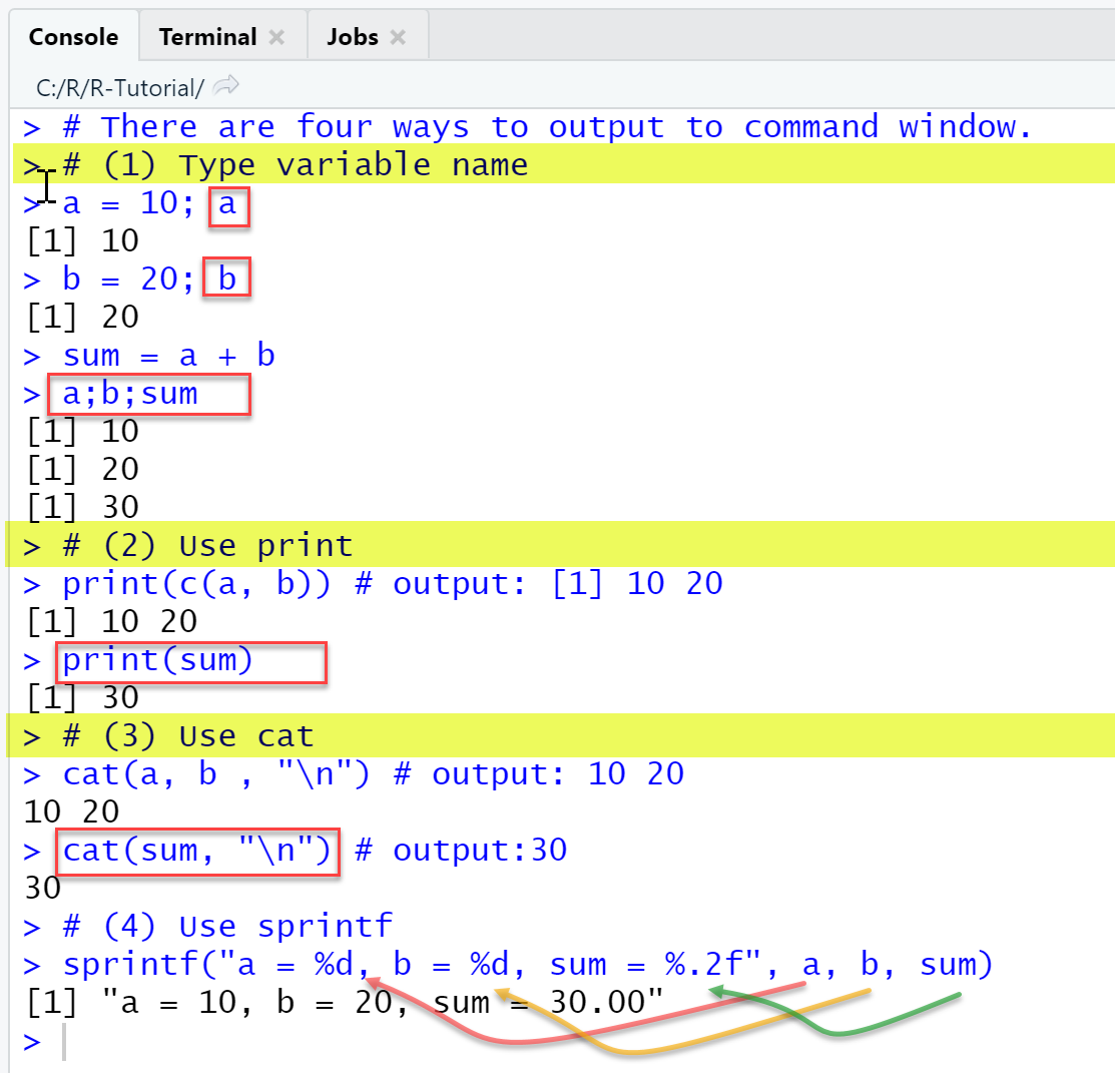
# There are four ways to output to command window
# (1) Type variable name 
a = 10; a
b = 20; b
sum = a + b
a; b; sum 
# (2) Use print
print(c(a, b)) # output: [1] 10 20
print(sum) 
# (3) Use cat
cat(a, b , "\n") # output: 10 20
cat(sum, "\n") # output:30
# (4) Use sprintf
sprintf("a = %d, b = %d, sum = %.2f", a, b, sum)

Output

RStudio Console Panel

When executing the script using the Run-menu item, output in console is as shown. In the test phase of new scripts we mostly just type the name of an object to see its content.
The function sprintf can be used when a more sophisticated formatting is required, with text and specification of decimal places. The placeholder %d (for integer), %f (for float) etc. specify a format for the data type of the corresponding variable. Take care that number and data type of variables match the placeholders.

Input from console

When presenting an R script to non-technical users, it can be helpful to let them enter configuration parameters as input from the console. Input entered in the console can be stored in variables using the readline-function. The readline-function receives as input argument a prompting text and returns the input as a string, even when numbers are entered. If the input is needed in other data formats, it must be converted using the corresponding functions as.numeric or as.integer. The script should be executed via Source, so that the prompt cursor is displayed and waits for user input.

Example: Input from console

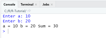
This example shows how to use the function readline to read input from console and store it in a variable. We read two values a and b, convert them to numerical values, and calculate their sum.

R Code: Input from console

Using readline with a prompt

prompt = 'Enter a: ' # Create a prompting text
a = readline(prompt) # Read input from console 

prompt = 'Enter b: ' # Create a prompting text
b = readline(prompt) # Read input from console 

sum = as.numeric(a) + as.numeric(b) # Calculate sum
cat("a =", a, "b =", b, "Sum =", sum) # Print to console

Output

RStudio Console Panel

When executing the script using the Source-menu item, output in console is as shown.

4. Control flow: Conditional statements and loops

Top

Control flow statements are used to determine depending on a condition which block of code to execute (conditional statements, if-else) or to execute a block of code repeatedly (loops: while, for, repeat) as long as a condition is satisfied. Control flow statements statements in R are pretty similar to those in

4-1 Conditional statements (if-else)

Conditional statements are used to control which of two or more statement blocks are executed depending on a condition. In R, as in most programming languages, they are implemented using the if-elseif-else-syntax, the elseif and else part being optional. The statements of a block are enclosed in braces, as shown in the syntax description.

Syntax: if-else

if (condition) {
    statement1
} else {
    statement2
}

Syntax: if-elseif-else

if (condition1) {
    statement1
} else if (condition2){
    statement2
} else {
	statement3
}

Example: Conditional statement

In this example we evaluate if a variable is positive, negative or zero and depending on the value of the variable a message is displayed.

R Code: Conditional statement

Determine if a number is positive / negative / zero

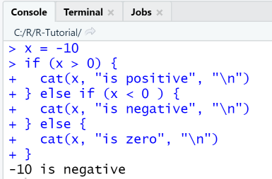
In line 5, the condition "x > 0" is evaluated: If true, the statement in line 3 is executed and the program flow continues in the first line after the if-else-statement. Else the next condition "x < 0" is evaluated and if true, the statement in line 5 is executed and the program flow continues in the first line after the if-else-statement. If none of the conditions is true, the default statement(s) in the "else"-part are executed.

x = -10
if (x > 0) {
  cat(x, "is positive")
} else if (x < 0 ) {
  cat(x, "is negative")
} else {
  cat(x, "is zero")
}

Output

RStudio Console Panel

When executing the script using the Run-menu item, output in console is as shown: The if-else command is a multi-line statement. In multiline statements, the first line has the >-symbol as prompt, and the following lines the +-symbol.

4-2 Loops

Loops are multiline statements which execute a block of code repeatedly as long as a condition is satisfied. R has three types of loops: while, for, repeat. Additionally, you can use the break and continue-commands to alter the normal execution flow of a loop, same as in other high level languages: with break, you leave the loop immediately, with continue, you skip an execution step. In R, loops are not used as frequently as in general-purpose programming languages. In R, most cases where you would need a loop in C or in Java, for example, calculate the sum of elements of a vector, are covered by a function.

While-Loop

A while loop allows statements to be executed repeatedly, as long as an execution condition is met. The variable that is queried in the condition is not automatically increased, so it must be explicitly incremented in the body of the loop. If there is no increase in the variable, the loop is executed endlessly.

Example: While-Loop

In this example we calculate the sum of the first 5 numbers: sum = 1+2+3+4+5 using a while-loop.

R-Code: While-Loop

Using while to calculate a sum

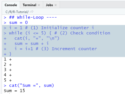
In line 3, a counter variable i is initialized with 1. In line 4 the loop condition "i <= 5" is checked. If "true", the statements in line 5-7 are executed (print the value of i, add the value of i to the value of sum, increment the value of i) and then the loop condition is checked again and the loop is repeated.

## While-Loop ----
sum = 0
i = 1 # (1) Initialize counter i  
while (i <= 5) { # (2) Check condition 
  cat(i, "+", "\n")
  sum = sum + i
  i = i+1 # (3) Increment counter     
}  
cat("Sum =", sum)

Output

RStudio Console Panel

When executing the script using the Run-menu item, output in console is as shown. Since the while-loop is a multi-line statement, the first line has the >-symbol as prompt, and the following lines the +-symbol.

For-Loop

A for-loop is a counting loop that defines a start and end condition for a counting variable (loop counter) and repeats a statement or a group of statements for a number of loop passes a specified by the loop counter. The loop counter is increased by 1 (or another step size) after each loop pass.

Example: For loop

In this example we calculate the sum of the first 5 numbers: sum = 1+2+3+4+5 using a for loop.

R Code: For loop

Using for-loop to calculate a sum

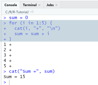
In this example, a counter variable i is initialized with 1. In line 3 the loop condition "i <= 5" is checked. If "true", the statements in line 4-5 are executed (print the value of i and add the value of i to the value of sum) then counter is incremented and the loop is repeated.

## For-Loop ----
sum = 0
for (i in 1:5) {
  cat(i, "+", "\n")
  sum = sum + i
}  
cat("Sum =", sum)

Output

RStudio Console Panel

When executing the script using the Run-menu item, output in console is as shown.

5. Vectors

Top

Vectors are one-dimensional indexed datastructures that store data as ordered collections of elements. Lists are a general form of vectors in which the various elements need not be of the same type, and are often themselves vectors or lists. New lists are created using the function list, as in mylist = list("apple", "pears", c(10, 20), TRUE).

A new empty vector of given length can be constructed via the function vector(mode, length) and preallocated with values using the function rep(), which creates repetitions. A vector then is filled with values with the concatenation-function c(). Vectors can be constructed by adding directly values to them using the c()-function, in this case, the R System will implicitly construct a vector with correct mode and length. The explicit creation of an empty vector with preallocation is useful when dealing with large data sets.

The parameter mode of the vector()-function specifies the type of the elements that the vector can contain, and can take values such as "logical", "numeric", "integer" or "list". The parameter length specifies the desired length of the vector.

x = vector(mode="numeric", length = 10) # optional!
x = c(1, 2, 3.5) # add elements using c()
n = length(x) # length of the vector is 3

Elements of a vector are accessed using an index that starts at 1. To access the i-th element in a vector x, we put the index in square brackets after the name of the vector, e.g. x[1] gives the first element, x[2] the second element and so on. Another way to index vectors in R is by using a character index; this will be treated more in depth in section DataFrames.

Vectors are created in different ways: by listing their elements explicitly using the c()-function, by combining existing vectors to a new vector, or by using special functions for creating sequences, repetitions or random numbers.

5-1 Create vectors using c()-function

Top

Vectors are created using the c()-function, which is used to combine values into a vector or list. For example, x = c(1, 4, 9, 16, 25) will create a numeric vector with five elements, and s = c("a", "b", "c") will create a string vector with 3 elements.

Example: Create and access vectors

This example shows how to create a vector using the c()-function and access its elements using the []-operator and indexes. Elements can be accessed in their original order or reverse order, through a single index, an index range or an index vector. A negative index is used to exclude specified elements.

R Code: Create and access vectors

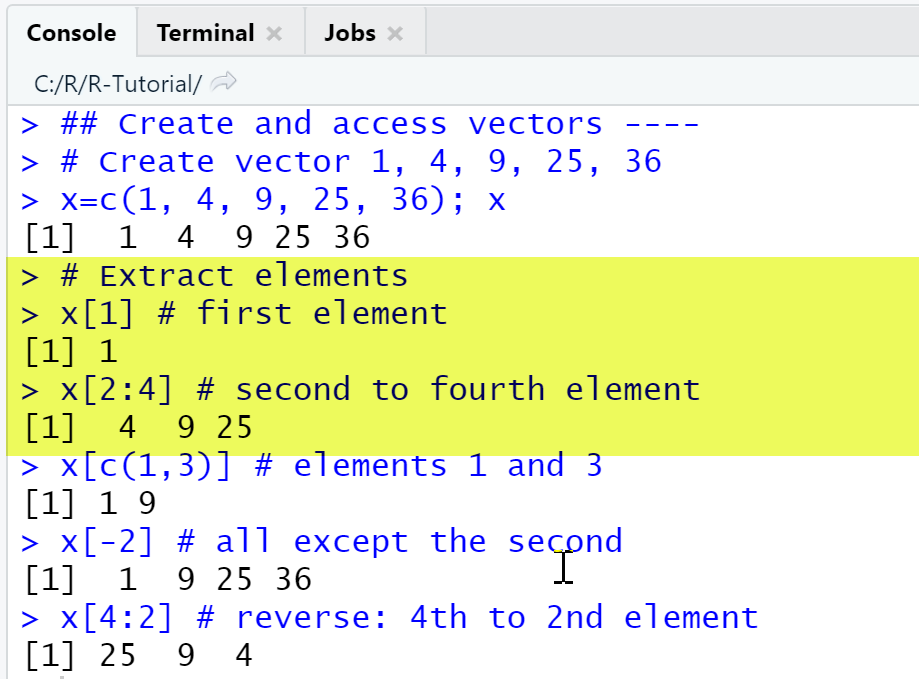
We first create a row vector with 5 elements, display the first element of the vector, then the second to fourth elements, then elements 1 and 3, then all elements except the second and finally show elements in reverse order.

# Create vector 1, 4, 9, 25, 36
x=c(1, 4, 9, 25, 36)
x
# Extract elements
x[1] # first element
x[2:4] # second to fourth element
x[c(1,3)] # elements 1 and 3
x[-2] # all except the second
x[4:2] # reverse: 4th to 2nd element

Output

RStudio Console Panel

5-2 Combine vectors to a new vector

Top

In R, two or more vectors can be combined using the c()-function: The statement c(x, y) appends the vector y to x. If the vectors have different data types and one of them is a character vector, they are both converted to data type character, so that the resulting vector has an unified data type.

Example: Combine vectors

In this example we create a numeric vector x and a character vector s and combine them into a new vector res.

R Code: Combine vectors

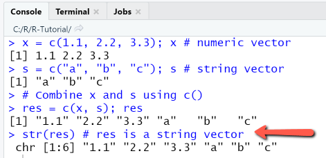
Combine two vectors using c()

x = c(1.1, 2.2, 3.3); x # numeric vector
s = c("a", "b", "c"); s # string vector
# Combine x and s using c()
res = c(x, s); res 
str(res) # res is a string vector

Output

RStudio Console Panel

5-3 Sequences and repetitions

Top

Regular sequences and repetitions of values are a special type of vectors, that are needed in statistical and numerical problems, for example the sequence 2,4,6,8,10 of even numbers that are smaller than 10, or 1, 1,1,1 as a four-time repetition of the number 1. R offers the possibility to generate sequences and repetitions using the functions seq() and rep() respectively. Another way to create sequences is the colon-operator, that can be used to create sequences with step size 1, for example, 1:10 creates the sequence of integers 1,2,...,10. The function seq(from, to, by, length.out, along.with) generates a sequence of numbers in a given interval [from, to] with given step size. The parameters by, length.out, along.with are optional, if they are not specified, default values are used. As an example, seq (2, 10, by = 2), generates the sequence of numbers with starting value 2, end value 10 and step size 2.

Example: Create sequences

The example shows how regular sequences of numbers are generated, either with the help of the colon-operator : or with the help of the seq() function.

R Code: Create sequences

Using the colon-operator and seq()

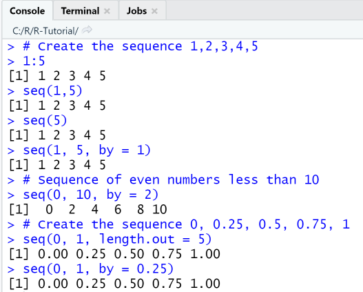
# Create the sequence 1,2,3,4,5
1:5  
seq(1,5) 
seq(5)
seq(1, 5, by = 1) 
# Sequence of even numbers less than 10 
seq(0, 10, by = 2)
# Create the sequence 0, 0.25, 0.5, 0.75, 1
seq(0, 1, length.out = 5)
seq(0, 1, by = 0.25)

Output

RStudio Console Panel

Example: Create repetitions

This example shows how to use the function rep() and its arguments to create a vector from repetitions of other objects. The function rep(x, times, length.out, each) replicates its first parameter x as specified by the other parameters: times - the number of replications of the vector, length.out - the length of the resulting vector, each - the number of replications per element.

R Code: Create repetitions

Using rep() and its parameters times, length.out, each

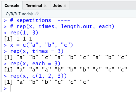
In order to repeat the value 1 three times, the function is called with rep(1, 3). If the first parameter x is a vector, this vector will be repeated three times. If the first parameter x is a vector and the value of the parameter each is set to 3, each element of the vector is repeated 3 times.

# Repetitions  ----
# rep(x, times, length.out, each)
rep(1, 3)
x = c("a", "b", "c")
rep(x, times = 3)
rep(x, each = 3)
rep(x, c(1, 2, 3))

Output

RStudio Console Panel

5-4 Vector operations

Top

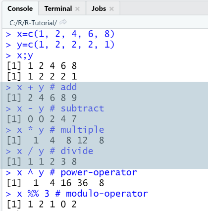
In R, all vector and matrix operations are performed element-by-element by default. Common vector operations are the arithmetic operations (+ ,-, *, /), the power-operation (^), and the modulo-operator (%%), that calculates the remainder of its operands. The result of a vector operation is a new vector with the same length as its operands.

Example: Vector operations

This example declares two vectors x and y with the same number of elements, then adds / subtracts / multiplies / divides them, calculates x at power y and x modulo y.

R Code: Vector operations

Using elementwise arithmetic operations

x=c(1, 2, 4, 6, 8)
y=c(1, 2, 2, 2, 1)
x;y
x + y # add
x - y # subtract
x * y # multiple
x / y # divide
x ^ y # power-operator
x %% 3 # modulo-operator

Output

RStudio Console Panel

5-5 Functions operating on vectors

Top

Firstly, the size of a vector is determined using the function length. Note that this function works only on vectors! For matrices, you must use the functions dim, nrow and ncol. Secondly, R contains a large number of elementary functions required for statistical computations, that all operate on vectors as well as on matrices: such as min, max, mean, var etc., also all commonly needed mathematical functions: exponential, logarithmic and trigonometric. Other utility functions are sort - for sorting a vector and summary for printing a table with its statistical properties. The summary() function delivers various statistical figures for an object and is used to get an initial overview on statistical properties of a data set, such as minimum, maximum, mean value etc.

Example: Vector functions

In this example we show the usage of selected statistical functions that take a vector as parameter.

R Code: Vector functions

Using sort, min, max, mean, etc.

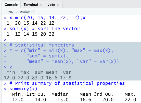
First, we create a new vector and sort it. Then we calculate some of its statistical properties and combine them in a new vector z. Finally, we print the default summary of its statistical properties as provided by the summary-function.

x = c(20, 15, 14, 22, 12);x
sort(x) # sort the vector

# Statistical functions
z = c("min" = min(x), "max" = max(x), 
      "sum" = sum(x), 
      "mean" = mean(x), "var" = var(x))
z
# Print summary of statistical properties
summary(x)

Output

RStudio Console Panel

6. Matrices

Top

Arrays are multi-dimensional generalizations of vectors, i.e. they are vectors that can be indexed by two or more indices. Arrays in R are created using the function array(data_vector, dim = dim_vector), for example array(1:24, dim=c(3,4,2)) creates an array with dimensions 2x3x4 that is filled with the numbers from 1 to 24.

Most commonly, we will need a special case of arrays, namely two-dimensional matrices to represent tabular data. Informally, a matrix can be viewed as a collection of elements of the same data type arranged in a two-dimensional rectangular layout. Matrices in R are created using the function matrix, or by combining vectors using the functions cbind and rbind, or simply using loops.

6-1 Create matrix using function matrix

Top

The first way to construct matrices in R is by using the function matrix(data, nrow, ncol, byrow = FALSE, dimnames), that takes as first argument the data used to fill the matrix, as second and third argument the number of rows /columns, and as fourth argument a parameter that specifies if the matrix is to be filled by row or by column. By default, matrices in R are created by column. If the provided data vector contains less elements than those nrow x ncol required for filling the matrix, the recycling rule applies: the existing elements are simply recycled.

Example: Create matrix

In this example we create a matrix with two rows and three columns: first from a vector with 6 elements, in the default by-column way, then from the same vector with 6 elements, but this time by row, and lastly from a vector with 3 elements, by column.

R Code: Create matrix

Using matrix-function

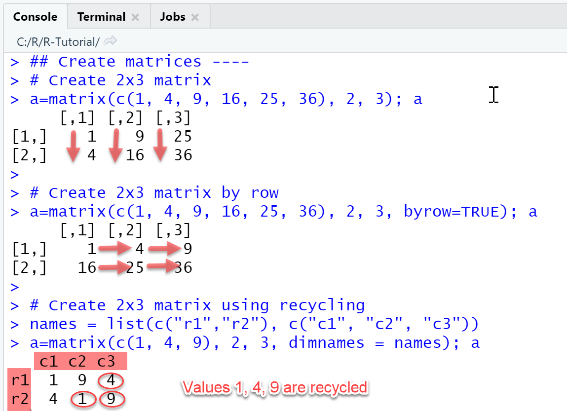
Line 2: Create matrix "a" from vector 1, 4, ..., 36.
Line 8: Create a list of names to be used as row names ("r1", "r2") and column names ("c1", "c2", "c3").
Line 9: Create matrix "a" with row and column names by assigning the previously created list to the parameter dimnames.

# Create 2x3 matrix
a=matrix(c(1, 4, 9, 16, 25, 36), 2, 3); a

# Create 2x3 matrix by row
a=matrix(c(1, 4, 9, 16, 25, 36), 2, 3, byrow=TRUE); a

# Create 2x3 matrix using recycling
names = list(c("r1","r2"), c("c1", "c2", "c3")) 
a=matrix(c(1, 4, 9), 2, 3, dimnames = names); a

Output

RStudio Console Panel

If a matrix is created without assigning row / column names explicitly, R will display as default a numbering in the form [i, ] for rows and [, j] for columns, as in the screenshot.

6-2 Create matrix by combining vectors

Top

Another way to create matrices in R is by combining vectors using the functions cbind() and rbind(). The function cbind is also used to append columns to a matrix; similarly, rbind is used to append rows to a matrix. More generally, these functions are used to combine vectors, matrices and data frames with matching dimensions, either as columns, or as rows. The two functions can als be nested to create a matrix out of building blocks, as in rbind(cbind(diag(2), 2*diag(2)), 3*diag(4)).

Example: Create matrix

Create matrix by combining vectors

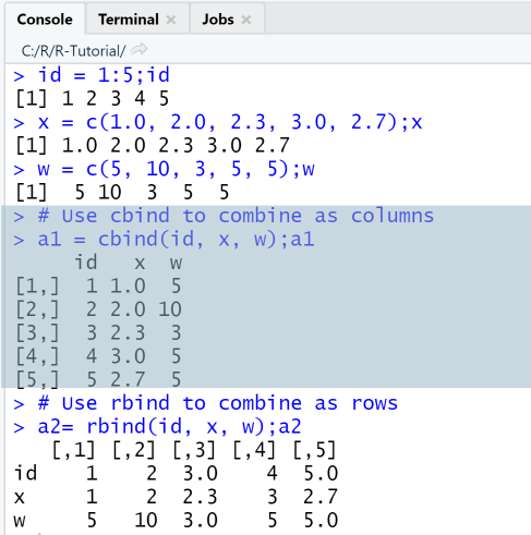
In this example we first define three vectors id, x and w, that store the data of exam gradings: id contains the module IDs, x contains the grades, w the weights (credit points) of a single module. Then we use the function cbind create a new matrix whose columns are the vectors id, x and w, and the function rbind to create a new matrix whose rows are the vectors id, x and w.

id = 1:5;id
x = c(1.0, 2.0, 2.3, 3.0, 2.7);x
w = c(5, 10, 3, 5, 5);w
# Use cbind to combine as columns
a1 = cbind(id, x, w);a1
# Use rbind to combine as rows
a2= rbind(id, x, w);a2

Output

RStudio Console Panel

6-3 Access elements of a matrix

Top

A matrix uses two indices: the first index denotes the row position and the second the column position of an element. The elements of a matrix a are accessed by writing the indices in brackets after the name of the matrix, separated by comma. Elements can also be extracted by applying a filter to a named row or column.

a[i, j] extracts the element at row i and column j.
a[3, ] extracts the third row
a[i1:i2, j1:j2] extracts the submatrix given by rows i1 to i2 and columns j1 to j2.
a[w==5, ] extracts all rows with the property that column w has value equal 5.
a[w==5 & x < 2, ] extracts all rows with the property that column w has value equal 5 and column x has value less than 2.

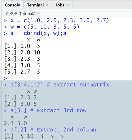
Example: Extract elements

Extract elements from matrix

In this example we first create a matrix with 5 rows and 2 columns and then extract elements, rows, columns or a submatrix.

x = c(1.0, 2.0, 2.3, 3.0, 2.7)
w = c(5, 10, 3, 5, 5)
a = cbind(x, w);a

a[3:4,1:2] # Extract submatrix
a[3,] # Extract 3rd row
a[,2] # Extract 2nd column

Output

6-4 Matrix operations and functions

The standard matrix operations (+, -, *, -, ^, %) are carried out elementwise, this is same as for vectors. The dimensions of a matrix "a" can be determined using the functions dim(a), nrow(a) and ncol(a).

Aside from the elementwise matrix operations, R supports algebraic matrix operations. The calculation of the determinant of a square matrix "a" is done using the function det(a), its inverse is calculated using the function solve(a), and its eigenvalues and eigenvectors using the function eigen(a). For the algebraic multiplication of two matrices "a" and "b", R has a somewhat complicated solution, namely the operator %*%, so a %*% b is the matrix product of a and b. Here a list of further useful matrix functions:

t(a) - transpose of a
diag(a) - returns the diagonal of a. The function diag is also used to create the identity matrix, for example diag(3) creates the 3x3 identity matrix.
rowmeans(a) - row means of a
colmeans(a) - column means of a

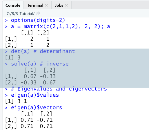
Example: Algebraic operations

Calculate determinant, inverse and eigenvalues

In this example we first create a square matrix with 2 rows and 2 columns and then calculate its determinant, inverse, eigenvalues and eigenvectors.

a = matrix(c(2,1,1,2), 2, 2); a
det(a) # determinant
solve(a) # inverse
# Eigenvalues and eigenvectors
eigen(a)$values 
eigen(a)$vectors

Output

RStudio Console Panel

7. Data Frames

Top

The third most important data structure in R is the data frame, which is useful especially when reading data from external files such as spreadsheets or databases. Dataframes store data in a spreadsheet-like structure, that is, like a table where the columns represent named variables and the rows named observations. The columns can have different data types, but the elements within a columns must have the same data type. Data frames are constructed in R using the function data.frame, either from columns / variables, or from a matrix, or by importing external data from files. Elements, columns and rows of a data frame can be accessed using different operators [], [[]], $. Rows and columns can be added using the functions cbind and rbind and removed using the function c().

7-1 Create data frame from column vectors

Top

The first way to construct data frames is by using the function data.frame and specifying the column vectors that represent the variables of the data set. The names of the vectors will become the column headers of the data frame.

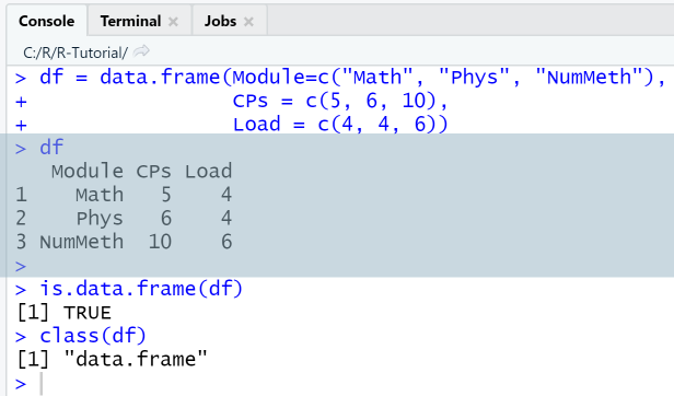
Example: Create data frame from column vectors

Use function data.frame

This example shows how to create a data frame from three column vectors, the first containing the name of modules, the second the credit points assigned to each module, and the third the workload for each module. The named variables here are "Module", "CPs" and "Load", and the observations are numbered with row numbers 1, 2 and 3.

df = data.frame(Module=c("Math", "Phys", "NumMeth"),
                CPs = c(5, 6, 10),
                Load = c(4, 4, 6))
df

is.data.frame(df)
class(df)

Output

RStudio Console Panel after executing "Run"

7-2 Create data frame from matrix

Top

Another way to create a new data frame using the function data.frame is by passing it a matrix as parameter. The row headers of the data frame can be specified using the parameter rowNames and the column headers by using the function names.

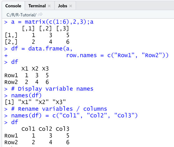
Example: Create data frame from matrix

Using functions data.frame and names

This example shows how to create a data frame from a 2x3 matrix using the function data.frame and specifying the row names as parameter of the function. The default variable names supplied by the function are X1, X2 and X3. Next, we rename the variable / column names using the function names.

a = matrix(c(1:6),2,3);a
df = data.frame(a, 
                row.names = c("Row1", "Row2"))
df
# Display variable names
names(df) 
# Rename variables / columns
names(df) = c("Col1", "Col2", "Col3") 
df

Output

RStudio Console Panel after executing "Run"

7-3 Access elements: slicing and subsetting

Top

For accessing elements of a data frame the operators [], [[]], $ can be used, that work similarly, but return different data objects.

Firstly, elements of a dataframe df are accessed in matrix-style by writing the row and column indices in brackets after the name of the data frame, separated by comma. This will return a data frame. For example, df[1:2, 3] extracts the first two rows and third column from data frame df and returns them as data frame. Elements can also be extracted by applying a filter to a named row or column.

Secondly, elements of a dataframe df can be accessed in list style using the [[]]-operator or the $-operator. In order to extract a column / variable, we put the quoted columns name in two square brackets after the data frame name, as in df[["Load"]]. Or, if using the $-sign, we simply write: df$Load. Both expressions return the third column from the data frame in the next example.

A third way to extract a subset of a data frame is by using the function subset(), which return subsets of vectors, matrices or data frames meeting given conditions. For example subset(df, df$Load == 4) would return the rows with Load equal to 4, that is, the first and second row.

Example: Access elements in data frame

This example shows how to access elements in a data frame. We use the same data frame "Modules" as in 7-1, its first variable containing the name of modules, the second variable the credit points assigned to each module, and the third variable the workload for each module.

R Code: Access elements in data frame

Using [], [[]] and $

We first create a data frame, then extract the third column "Load" containing the workload using both matrix- and list-style operators.

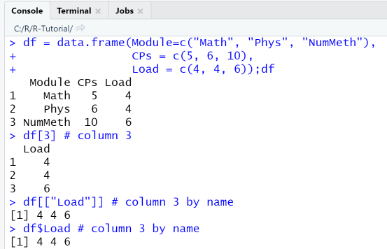
df = data.frame(Module=c("Math", "Phys", "NumMeth"),
                CPs = c(5, 6, 10),
                Load = c(4, 4, 6));df
df[3] # column 3
df[["Load"]] # column 3 by name
df$Load # column 3 by name

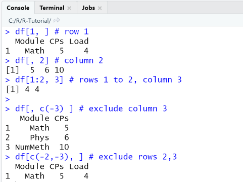
When extracting a row or a range of rows, the place after the comma, which represents the column index, must be left empty (means: all columns) or contain the selected column indices. Similarly, when extracting a column or a range of columns, the place before the comma, which represents the row index, must be left empty (means: all rows) or contain the selected row indices. Negative indices are used to remove rows and columns from a data frame: df[, c(-3] removes the 2nd and 3rd column, df[c(-2,-3), ] removes the 2nd and 3rd row.

df[1, ] # row 1
df[, 2] # column 2
df[1:2, 3] # rows 1 to 2, column 3

df[, c(-3) ] # exclude column 3
df[c(-2,-3), ] # exclude rows 2,3

Output

RStudio Console Panel after executing "Run"

Observe that df[3] returns a data frame, which is evident from the row numbering, while df[["Load"]] and df$Load return the same column as vector.

In the second code fragment we use only matrix-style operations to extract subsets of the data frame.

7-4 Add /remove columns and rows

Top

After creating a data frame, it may be required to add additional rows and columns. This is done by creating vectors of matching length and appending them using the functions cbind for columns and rbind for rows. Note that the new columns or rows are always appended at the end, after the last row or column. If an insertion at a specific index is needed, rbind must be used in combination with some re-indexing.

Example: Add and remove columns and rows

Using functions cbind, rbind and c()

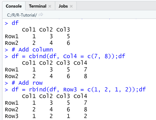
This example uses the 2x3 data frame constructed from a matrix that we created in the previous example. First, a column is appended to df and the original dataframe df is replaced by the new one. Then, a row is appended to df, so the data frame has now three rows and 4 columns.

df 
# Add column
df = cbind(df, Col4 = c(7, 8));df 
# Add row
df = rbind(df, Row3 = c(1, 2, 1, 2));df

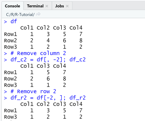
Next, we remove column 2 from the data frame df by using the negative index df[-2] and store the result in the new data frame df_c2. Finally, we remove row 2 from the data frame df by using the negative index df[-2, ].

df 
# Remove column 2 
df_c2 = df[, -2]; df_c2 
# Remove row 2
df_r2 = df[-2, ]; df_r2

Output

RStudio Console Panel after executing "Run"

7-5 Import data from files

Top

When working on statistical and data science projects, the data usually are external and must be imported from files or databases. R supports data import from external sources via the functions read.table, read.csv and read.csv2, which all import data from an external file, specified through its path, into a data frame. The functions read.csv and read.csv2 are derived from read.table, and differ in that they have other default settings for their arguments. The difference between read.csv and read.csv2 is minor: read.csv is used for data where commas are used as separators and periods are used as decimals, while read.csv2 is for data where semicolons are used as separators and commas are used as decimals. So the latter is more frequently used in European countries. The import from other data sources is supported through a number of libraries: import from Excel-files through the library XLConnect import from JSON through the library rjson etc.

So which import function is best to use when? If your data is in a plain text file, with tab as a column delimiter, use the function read.table. Else, if your data is in a csv-file, with comma as a column delimiter, use the function read.csv. Else, if your data is in a csv-file, with semicolon as a column delimiter, use the function read.csv2.

Before importing external data from a text or csv-file, the following should be checked:

Folder: If the file to be imported is placed in the current R working directory, it can be specified through its filename alone, for example read.table("modules.txt"). Else you must specify a relative path according to the rules of your operating system.
Encoding: If your file is encoded in UTF8 using Byte Order Mark (BOM), this will appear as weird symbols at the beginning. Either change the encoding, or import with option fileEncoding = "UTF-8-BOM".
End-of-line: Each line must end with an end-of-line character, else the import will generate an error. You can check and fix this using a text editor such as Notepad++.
Separator: The default separator for read.table is the tab. If yor data uses other separators, such as comma or semicolon, you should use the functions read.csv or read.csv2.

Import data using read.table

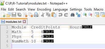In this example we use read.table with different options to import data from the file modules.txt that contains tabular data with columns separated by tabs. We put the file in our R working directory and use Notepad++ to check the correct enconding, tab separator and end-of-lines.

Example: Import data from text files

Using function read.table

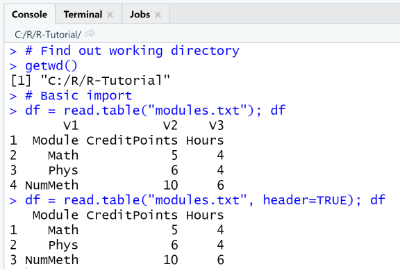
First, we check the working directory with getwd() and make sure to place the file in that directory. Then, we call read.table in the most basic setting, by passing it only the file name as argument. Next, we call read.table with the option header=TRUE, so that the first line of the file is interpreted as header.

getwd() 
# Basic import
df = read.table("modules.txt"); df 
df = read.table("modules.txt", header=TRUE); df

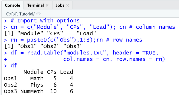
Finally, we call read.table with custom options for the arguments header, colnames, and rownames so that we can rename the default row and column names from the file. In line 2 we create a vector with new column names, that we use with the option col.names to replace the default column names that were imported due to the option header = TRUE. In line 3 we create a vector with new row names, that we use with the option row.names to replace the default row numbering.

# Import with options
cn = c("Module", "CPs", "Load"); cn # column names
rn = paste0(c("Obs"),1:3); rn # row names
df = read.table("modules.txt", header = TRUE,
                col.names = cn, row.names = rn)
df

Output

RStudio Console Panel after executing "Run"

Note that the data frame df created from the basic import has received the default variable names V1, V2 and V3 and row numbers 1, 2, 3. The first line in the file was considered as being an observation rather than a header line, this is because the default setting for headers in read.table is header = FALSE, that is the function assumes a data file with no headers.

The advanced import with options enables to change the default row and column names.

Import data using read.csv

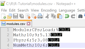In this example we use read.csv and read.csv2 with basic and advanced options to import data from the file modules.csv that contains tabular data with columns separated by semicolon and comma as a decimal delimiter. The name of the last column is an invalid R name and the last row contains a missing value, these are things to be considered when importing from files. We put the file in our R working directory and use Notepad++ to check the correct enconding, separator and end-of-lines.

The functions read.csv and read.csv2 have a number of options, here a selection:

header - specify if the first line in the file should be interpreted as column headers
fileEncoding - specifies the file encoding of the file: this is useful if the encoding of your file is different than what R expects.
column.names - set the column names of the data frame: this is useful when the file has no header or the header should be overwritten
row.names - set the row names of the data frame: this is useful if you need other row names than the default line numbers.
colClasses - specify the data types of all or selected columns.

Example: Import data from csv-files

Using functions read.csv and read.csv2

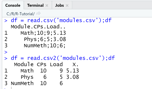
The first attempt with read.csv('modules.csv') fails to import the data correctly since our data uses the semicolon as delimiter, not comma as specified in the default for read.csv. The second attempt with read.csv2('modules.csv') imports the data correctly, however, the column name "%" for the last column is not imported correctly since it is is not a valid name in R, so the import generated another column name instead..

df = read.csv('modules.csv');df
df = read.csv2('modules.csv');df

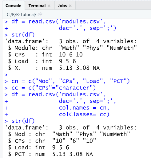
Next, we import the same data file using the function read.csv and specifiying the correct delimiter and separator. The import succeeds, however the last column name has been changed. Next, we change the column names and the data type of the column CPs. The changes can be checked using the function str, that shows the structure of the data frame.

df = read.csv('modules.csv', 
              dec='.', sep=';')
str(df)

cn = c("Mod", "CPs", "Load", "PCT")
cc = c("CPs"="character")
df = read.csv('modules.csv', 
              dec='.', sep=';', 
              col.names = cn,
              colClasses= cc)
str(df)

Output

RStudio Console Panel after executing "Run"

First import with read.csv fails, second import with read.csv2 succeeds.

The internal structure of the data frame df as displayed by the str-function shows that the data type of column CPs has successfully been changed to "character". Note that since the data type for the column CPs was specified as character, the numbers are displayed with quotation marks.

8. Functions

Top

A function is a group of instructions that is only executed when it is called. Functions are defined once and can then be called as often as required; functions may have parameters or not and also may return values or not. The most frequent application of functions in R is to use built-in R-functions such as sin, cos, min, max, plot, etc. With advanced R programming, when developing larger projects, it is an advisable practice to structure them using user-defined functions, or to develop own functions for own tasks.

8-1 R built-in functions

Top

The R framework has a broad range of built-in functions for different tasks, that can be used without importing additional libraries. So before programming own functions, it is advisable to check the existing R functions. R functions are generic, which means that they work on all type of arguments: with print, you can display any type of object, not only variables. R functions also tend to have long lists of arguments. The first arguments in the parameter list are usually the most important ones, other arguments are optional and have default values.

Output and input: print, cat, sprintf
Object creation: c, list, vector, matrix, data.frame, seq, rep ...
Object verification: is.integer, is.vector, is.matrix, ...
Object composition: cbind, rbind, ...
Typecasting: as.integer, as.vector, as.matrix, ...
Object structure and summaries: typeof, class, str, summary, dim, head, tail
Mathematical: abs, sqrt, ceiling, floor, round, trunc, sin, cos, tan, log, exp
String manipulation: paste, grep, substr, sub
Statistical: mean, sd, median, range, sum, diff
Statistical, distributions: dnorm (density function), pnorm (cumulative distribution), qnorm (quantile function), dunif (continuous uniform density), punif (continuous uniform distribution), qunif (quantile function), ...

For example, if you need to create a vector of normally distributed numbers, you would have to look up the function rnorm(). To create a vector of n normally distributed elements with mean m and standard variation sd, you can use different function calls, depending on the requirements of your program. Best practice is to specify arguments as name-value pairs, so as to avoid errors.

rnorm(1000, 50, 15) # (1) specify arguments as values only
rnorm(1000, mean = 50, sd = 15) # (2) specify arguments as name-value pairs
vec = rnorm(n = 1000, mean = 50, sd = 15) # (3)store result in a vector

8-2 User defined functions

Top

User-defined functions must be defined before they can be called. The definition can be placed in the same script file where the function is used or in a separate R file. When using R functions, the following should be considered:

Before an user-defined function can be called, it must be loaded into the current R session using the Run or Source menu item, it then will appear in the Environment tab. A function that is saved in a separate R-script, for example myfun.R, must be included in the calling script with the command source(myfun.R).

In R, function arguments are passed by value. This means that the value of a function argument is not changed within the function. If values computed in the function body are needed in the calling function, they must be passed as return values.
When defining a function, it is possible to assign a default value to an argument, that is taken when the function call does not specify the value for that argument.

Function definition
Functions are defined by assigning the keyword "function" to the function name and then specifying a comma-separated list of arguments in round brackets and followed by the function body, ie declaration block of the function, that must be enclosed with braces.

Syntax: Function definition

function_name = function(arg1, arg2, ...) {
   # Function body: insert your statements here
}

Function calls
Function can be called in different ways, either by writing the function name, followed by a comma-separated list of actual arguments in round brackets, or by writing the function name, followed by a comma-separated list of argument-value assignments. If function calls are given arguments in the "arg=value" form, they may be placed in any order.

Syntax: Function calls

# Function with no return value
function_name(val1, val2, ...)
function_name(arg1 = val1, arg2 = val2, ...)
# Function with return value
ret = function_name(val1, val2, ...)
ret = function_name(arg1 = val1, arg2 = val2, ...)

Functions with no return value

Top

Functions with no return value are basically statements that depend on a number of arguments and can be called using the function name. They may be useful to create customized output or customized plots, as in the next example: we define a function myfun1 that has two arguments: a title for the object to be printed and the object itself, and these are combined to a nice output demarked with two separator lines.

Example: Function with no return value

Define and call a function for customized output

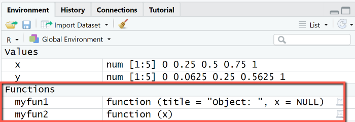
We first define a function myfun1 for customized output of an R object x by specifying the function name and the arguments (title and x), followed by the actual output statements grouped with braces. Both arguments receive default values: title has the default value "Object: " and x the NULL-object as default.

# 1. Define function
myfun1 = function(title = "Object: ", x = NULL) { 
  cat("====================================\n")
  cat(title);cat("\n")
  print(x)
  cat("====================================\n")
}

Then, we call the function multiple times and output a number, a vector and a matrix:

Line 2: only second argument is specified, as name-value pair.
Line 3 and 4: title and x are specified as name-value-pairs.
Line 5: title and x are specified as values, object x is a matrix.

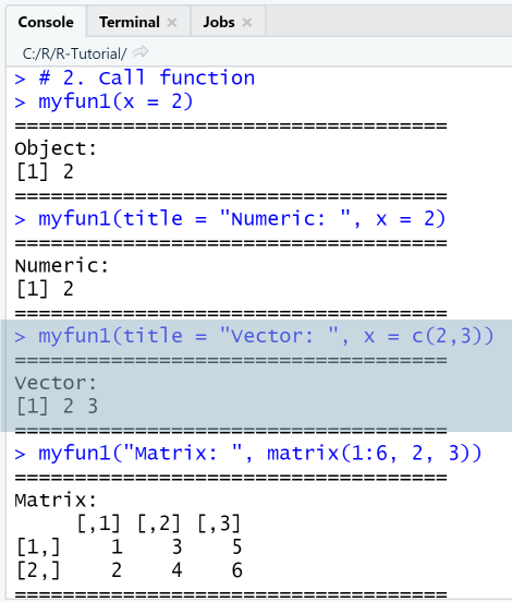
# 2. Call function
myfun1(x = 2)
myfun1(title = "Numeric: ", x = 2)
myfun1(title = "Vector: ", x = c(2,3))
myfun1("Matrix: ", matrix(1:6, 2, 3))

Output

RStudio Console Panel

In the first function call with x = 2, no value is provided for the argument title, so the default value "Object: " was taken.

Function with return value

Top

Functions with a return value calculate a new value or object using their arguments and return this for further usage in the calling function. The return values are specified with the keyword "return" and the subsequent return object, that must be put in round brackets. All instructions after the return line are ignored, i.e. return marks the end of the instructions in the function body. If no "return" is found, R takes the last statement line in the function body as the return value. This means that in R, the return statement can be omitted, it is however clearer to specify it explicitly.

Examples for functions with return values are all the usual mathematical and statistical functions (trigonometric, exponential, sum, mean etc.) In the next example we define a function myfun2 that calculates the square of its input argument and returns it to the calling function.

Example: Function with return value

Define and call a function y = myfun2(x)

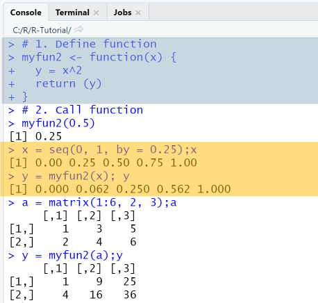
We first define the function myfun2 with the correct syntax by specifying the function name and the arguments, followed by the actual statements that we group with braces. Then we use the function to calculate the square of a a number, a sequence vector and a matrix.

# 1. Define function
myfun2 = function(x) { 
  y = x^2
  return (y)
} 
# 2. Call function
myfun2(0.5)
x = seq(0, 1, by = 0.25);x
y = myfun2(x); y
a = matrix(1:6, 2, 3);a
y = myfun2(a);y

Output

RStudio Console Panel

Binary Operators

Top

A binary operator is a shortcut for a function with two arguments and one return value. For example, the algebraic matrix multiplication in R is implemented as binary operator: it is more convenient to write A %*% B instead of multiply(A, B). Other functions that could be implemented as binary operators are: weighted sum of two vectors, adding a row or column to a data frame and returning the new dataframe. In R, a binary operator is created by defining the corresponding function and specifying the function name in the form '%op%', that is, surround the name of the operator with single quotes and percent symbols: Then, the binary operator can be used in the form x %op% y instead of using the function call %op%(x, y).

The next example shows how to create and use a binary operator %c+% that adds a column to a dataframe and resets the column names to the default values X1, X2, etc.

Example: Create and use a new binary operator

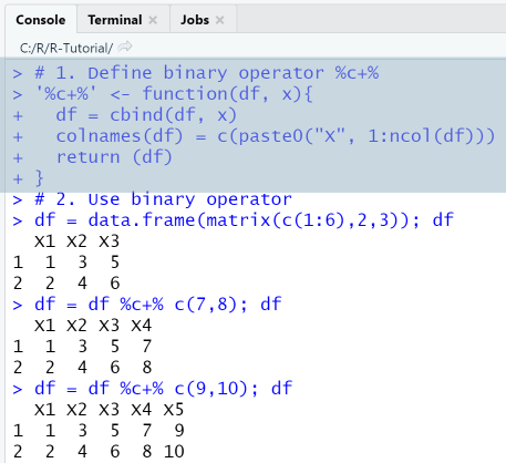
The binary operator %c+% is defined as function with the same name, just take care to surround the name with single quotes. The arguments of the function are: df - the data frame, and x - a column vector. In line 3 we append x to df using cbind, in line 4 we change the column names to be X1, X2, etc.

# 1. Define binary operator %c+%
'%c+%' = function(df, x){
  df = cbind(df, x)
  colnames(df) = c(paste0("X", 1:ncol(df)))
  return (df)
}

The usage of the binary operator is simply df %c+% x adds column x to data frame df. In order to test it, we first create a data frame from a 2x3 matrix, then add the column 7, 8 to it, and finally the column 9, 10.

# 2. Use binary operator
df = data.frame(matrix(c(1:6),2,3)); df
df = df %c+% c(7,8); df
df = df %c+% c(9,10); df

Output

RStudio Console Panel

9. Data visualization in R

Top

Data visualization is an important step of data analysis and R being a language designed specifically for statistical tasks, it has a strong support for data visualization. Graphics can be realized in R either through the built-in plotting functions, the generic function plot and its derivates hist, boxplot, barplot etc., or through the plotting capabilities of the package ggplot. The learning curve is steep, the challenge is not only to choose the correct visualization to answer your question, but also to choose between different packages.

Graphics in R and RStudio

Top

Before starting, we go through some basics about using graphics in RStudio. Graphics in RStudio are displayed by default in the Plots-Pane. The visualization is a bit hidden there. A better way to display graphics is by using the dev()-functions, that provide control over multiple graphics devices. With dev.new(), you can open a new device in RStudio, with dev.off() you shut down the currently active device, with graphics.off() you close all devices.

Graphics can be presented in a grid layout using the functions par and layout. The par-function together with its parameters mfrow and mfcol are used to create a matrix of plots in one plotting space. For example, par(mfrow=c(1,2)) creates a space with one row and two columns, where you can place two figures. The layout-function creates a grid layout, in which the plots are placed in the order specified by a layout matrix.

R Code: Graphics configuration

Using dev and layout

In this example we create a grid layout for four plot types used frequently in statistics: scatter plot, histogram, boxplot and barplot. The data that we plot are synthetic age and height data, that we generate using the known functions rep (for repetitions) and rnorm (for normally distributed numbers).

dev.new()
layout.matrix = matrix(c(1, 3, 2, 4), nrow=2, ncol=2)
layout(mat = layout.matrix,
       heights = c(2, 2), # Heights of the two rows
       widths = c(2, 2)) # Widths of the two columns
layout.show(4)
age = c(rep(20, 10), rep(30, 5), rep(40, 5))
height = rnorm(20, mean=170, sd=5)
df = data.frame(Age = age, Height=height)
plot(x=df$Age,y=df$Height, main="Scatterplot: Height vs. Age")
hist(df$Height, main="Histogram: Height")
barplot(height=table(df$Age), main = "Barplot: Age count")
boxplot(df$Height, main="Boxplot: Height")

Output

Graphics device with 2x2 layout

Since the functions plot, hist, boxplot and barplot were called with only the basic arguments and no further configuration, the plots are shown with their default layout.

9-1 Preparation: Choose a data set for testing

Top

For our visualizations, we use the data set demo_data.csv containing demographic data, with a total of 200 observations for six variables (Age, Height, Weight, BMI, BMI Category, Gender), 100 men and 100 female. Two of the variables (BMI Category and Gender) are categorical, the other numerical. The task is to visualize height, weight and body-mass-index (BMI) at different ages and compare the genders.

Data sets used in real-life R projects are imported from external data sources (files and data bases) into data frames (observations of multiple variables). R also has a number of pre-loaded data sets, for example mtcars - Motor Trend Car Road Tests, nhtemp - Average Yearly Temperatures in New Haven and many others. A list of built-in data sets can be printed with the command data(), to load one of them, the same command can be used, ie data(mtcar) loads the mtcar data set. Other data sets can be installed and imported as library, one such example is the National Health and Nutrition Examination Survey (NHANES) dataset, that contains demographic and health data.

R Code: Prepare demo data set

Using read.csv, str, subset

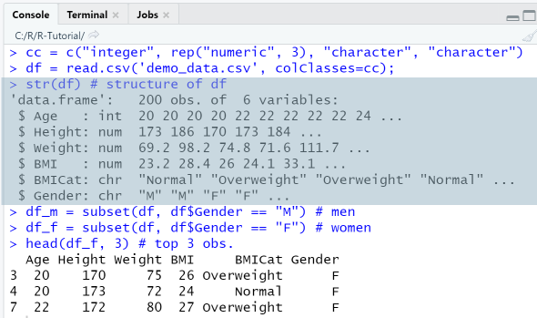
The data are available as csv-file and must be imported using the known function read.csv, with the option colClasses for specifying the data types. After importing them, we check the structure of the data frames with str. Finally, we extract using subset two data frames df_m and df_f that contain womens and men's data, respectively.

cc = c("integer", rep("numeric", 3), "character", "character")
df = read.csv('demo_data.csv', colClasses=cc);
str(df) # structure of df
df_m = subset(df, df$Gender == "M") # men
df_f = subset(df, df$Gender == "F") # women
head(df_f, 3) # top 3 obs.

Output

RStudio Console Panel

9-2 Scatter plot: find out trends and correlations

Top

Scatter plots are frequently used in a data analysis project: they show raw data, one variable (y-axis) vs. another (x-axis) as data points, which results in a scattered appearance, hence the name. Often, a regression line is added, to determine if the variable shows a trend. When plotting multiple y-variables against the same x-axis, the plot is visually enhanced with colors and symbols. If the data are grouped in clusters, it is safe to assume that they exhibit correlations, if they are randomly scattered all over the space, they will be independent and without correlation.

The generic function for 2-dimensional plotting in R is the plot-function, with syntax plot(x, y, type, main, xlab, ylab, col, pch, cex...). The data and configuration options for the plot are specified using arguments, the most important being:

x and y are the coordinates of the points to be plotted. The most basic usage is plot(x, y) where, x and y are two vectors. An alternative usage is to specify an R object / data frame as x-coordinates; in this case, the y argument is optional.
type is the type of the plot ("p" - points, "l" - lines, "h"-histogram, ...),
main is the main title of the plot,
xlab and ylab are the x- and y-labels, respectively,
xlim and ylim are the limits for the x- and y-axes, respectively,
col is used to specify the colors for title, labels, symbols.
pch is used to specify the symbol type. Symbols can be specified through a number code (1, 2, ...) or the symbol itself (o, *, ...).
cex is used to specify the font size for title, labels, symbols.

The legend-function is used to create a legend and has the syntax legend(x, legend, fill, col, lty, lwd, pch, ...), where x is a position that can be specified as string, legend is the text to be displayed, fill specifies the colors for filling the boxes, col specifies the colors of points or lines, lty the line type and pch the symbols for the plots. The argument bty specifies if the legend rectangle should have a border or not.

The text-function adds text to a plot. Its syntax is text(x, y, labels), where x and y are coordinate vectors where the text labels should be written.

Example: Scatter plot of two variables

This example shows how to create a scatter plot of two variables on a new graphics device and use the available options for specifying all the details that make a plot informative: title, axis labels, plot type, symbols and legend.

R Code: Scatter plot of two variables

Usage of plot, lines and legend

dev.new() 
c = c("deepskyblue", "darkorange") # colors
s = c(17, 19) # symbols: triangle = 17, circle = 19
plot(df_m$Age, df_m$Height, main="Height (men vs women)", 
     xlim = c(20, 80), ylim=c(140, 200), panel.first=grid(),
     xlab="Age", ylab="Height", col=c[1], pch = s[1], cex=1.1)
lines(df_m$Age, df_f$Height, type="p", col=c[2], pch = s[2], cex = 1.2)
legend("topleft", legend=c("Men", "Women"), 
       lty = c("blank","blank"),  # line type
       col = c, pch = s, # colors and symbols
       bty = "y") # border

Line 1: dev.new() opens a new graphics device.
Line 2-3: Create vectors for the colors and symbols to be used.
Line 4-6: The first plot for the male BMI is created using the plot-function. The x-coordinates are obtained from the column Age of data frame df_m, the y-coordinates from column BMI of data frame df_m. We specify title, x-labels and y-labels.
Line 7: A second plot of type "points" is added to the figure using the lines-function: here we set as y coordinates the column df_f$BMI.
Line 8-11: Create a legend in the topleft corner. Note that symbols and colors match those of the two plots.

Output

RStudio Graphics Device: Height by age

The first scatterplot shows that in this data sample men and women heights are loosely grouped in two clusters, and most men are taller than most women, possibly by some factor. The plot also gives an idea of the ranges for men's and women's height, and eventual outliers. This plot, however, does not show what the mean height of men / women is, or the distribution of the variables.

Example: Scatter plot with trend line

This example shows how to create scatter plots with added trend lines using the functions plot, abline and lm. A linear regression model for two variables x and y can be created with lm(y~x), which returns an object containing the coefficients of the regression line. This then can be passed as argument to the abline -function.

R Code: Scatter plot of two variables

Usage of plot, abline, lm

Line 1-2: Define vectors for the colors and symbols to be used.
Line 3: Specify a plotting space with one row and two columns.
Line 4-6: Add a scatter plot for men's weights using plot-function. Specify title, axis limits, labels, color etc.
Line 8-10: A second scatter plot for female weight is created and placed on the right-hand plotting space.
Line 7 and 11: Add trend lines for men's / women's weights using the functions abline and lm.

c = c("deepskyblue", "darkorange") # colors
s = c(17, 19) # symbols: triangle = 17, circle = 19
par(mfrow=c(1, 2))
plot(df_m$Age, df_m$Weight, main="Weight vs Age (men)", 
     xlim = c(20, 80),  panel.first=grid(),
     xlab="Age", ylab="Weight", col=c[1], pch = s[1], cex=1.1)
abline(lm(df_m$Weight~df_m$Age),  col=c[1], lwd = 2)
plot(df_f$Age, df_f$Weight, main="Weight vs Age (women)", 
     xlim = c(20, 80),  panel.first=grid(),
     xlab="Age", ylab="Weight", col=c[2], pch = s[2], cex=1.1)
abline(lm(df_f$Weight~df_f$Age), col=c[2], lwd = 2)

Output

RStudio Graphics Device: Weight by age

The weight of both men and women in the sample population increases slightly with age, as the trend lines show.

9-3 Histogram: display frequency distribution of variables

Top

A histogram is the graphic representation of the frequency distribution of a variable. The data of the variable are sorted according to their size and divided into a number of classes or bins that can, but do not have to be, of the same width. A rectangle is drawn above each class, the area of which is proportional to the frequency of this class. A histogram can be a frequency plot (the area represents the count of elements in this class) or a density plot (the area represents the percentage of elements in this class).

The function for plotting histograms in R is hist(x, breaks, freq, probability, main, xlim, ylim, xlab, ylab) and it requires only one variable x as input, the frequencies being calculated from the variable. The freq-argument determines if the histogram is a frequency plot (freq=TRUE) or a density plot (freq=FALSE). The breaks-argument is used to specify the number of bins, either as number, i.e. breaks = 4, or as vector, breaks=c(15,20,25,30,35,40). Note that when you specify breaks as a number, the hist-function will use it only as a starting point for its division and the histogram will not have that exact number of bins. When specifying breaks as a column vector, the entire value range of the variable should be covered, and, in most cases, the partition should be equidistant, which makes the histogram easier for interpretation.

Example: Histograms (frequency / density)

This example shows how to create frequency and density histograms and add a normal distribution curve to the diagrams. The function dnorm(x, mean, sd) creates a normal distribution with given mean and standard deviation. This can be plotted as curve using the function curve.

R Code: Histograms (frequency / density)

Using hist, dnorm, curve

In line 2 we use the par-function with the argument mfrow=c(1, 2) to create a plotting space spanning one row and two columns. The histograms created next will be placed in sequence on the available space. We set the axes limits xlim and ylim to be identical, so as to make the comparison easier. With panel.first=grid() we add a grid to the plot.

dev.new()
par(mfrow=c(1, 2))
hist(df_m$Height, col="deepskyblue", xlab="Height (cm)",
     xlim = c(150, 200), ylim=c(0,50),
     main="Men's Height", panel.first=grid() )
hist(df_f$Height,  col="darkorange", xlab="Height (cm)", 
     xlim = c(150, 200), ylim=c(0,50),
     main="Women's Height", panel.first=grid() )

Next, we create two density histograms, this is obtained by setting freq=FALSE. The argument density creates shading lines of the specified density. To each histogram we add a curve plot of the normal distribution with mean and standard deviation of the corresponding variable.

hist(df_m$Height,  col="deepskyblue",
     freq=FALSE, density = 20, 
     xlab="Height (cm)", xlim = c(150, 200), 
     main="Height (men)", panel.first=grid() )
curve(dnorm(x, mean=mean(df_m$Height), sd=sd(df_m$Height)), 
      col=c[1], lwd=2, add=TRUE)
hist(df_f$Height,  col="darkorange", 
     freq=FALSE, density = 20, 
     xlab="Height (cm)", xlim = c(150, 200), 
     main="Height (women)", panel.first=grid() )
curve(dnorm(x, mean=mean(df_f$Height), sd=sd(df_f$Height)), 
      col=c[2], lwd=2, add=TRUE)

Output

RStudio Graphics Device: Height distribution

The frequency histogram visualization shows that the height variable in the population sample has a normal distribution, with a mean value of 175 for men and 170 for women. Women's heights range in between 150 and 185, men's height in between 160 and 195.

The density histogram visualization also shows that the height variable sample has a normal distribution, additionally, we can plot the normal distribution that fits the data. The area of the rectangles now is the fraction of data points falling into a cell, the sum of all areas adds up to 1.

In the previous example we used par to display the two histograms for men and women heights next to each other. Another way to visualize the distribution of two variables simultaneously is to plot them on the same axes using the add parameter of the hist-function. This visualization requires to specify the colors in rgb-form with transparency, in order to keep information for overlapping regions.

Example: Compare BMI distribution (male vs female)

Usage of hist, break and legend

In this example we create the BMI-histogram for men and women separately and on the same axis. First, we create a plotting space with one row and two columns and call the hist-function twice with the default breaks-setting.

par(mfrow=c(1, 2))
c = c(rgb(0,0.6,1,0.5), rgb(1,0.6,0,0.8)) # colors
hist(df_m$BMI, 
     col=c[1], xlim=c(15,40), 
     xlab="BMI",  main="BMI (men)" )
hist(df_f$BMI, 
     col=c[2], xlim=c(15,40),
     xlab="BMI",  main="BMI (women)" )
mtext("Histograms", side = 3, line = -1, outer = TRUE, cex = 1.3)

Next, we show the histograms for male and female BMI distribution on the same diagram, with overlapping regions, using the add argument, that we set to "TRUE". The breaks-parameter is set to an equidistant column vector. The colors are specified as rgb-values with transparency, the legend is added in the topright corner.

c = c(rgb(0,0.6,1,0.5), rgb(1,0.6,0,0.8)) # colors
b = c(15,20,25,30,35,40) # equidistant breaks
hist(df_m$BMI, breaks=b, 
     col=c[1], xlim=c(15,40), ylim = c(0, 60),
     xlab="BMI", ylab="Count", main="BMI distribution (men / women)" )
hist(df_f$BMI, breaks=b, 
     col=c[2], xlim=c(15,40), ylim = c(0, 60),
     add=TRUE )
legend("topright", legend=c("Men", "Women"), fill = c)

Output

RStudio Device

The hist-function has split the domain of the variable df_m$BMI, which is [20, 36], in 8 equal bins. We observe that the third rectangle [24, 26] is heighest, which means that most men (n=2*30 = 60) in the sample have a BMI between 24 and 26.

The histogram with overlapping has only five bins, that roughly correspond to a classification in underweight, normal, slightly overweight, overweight and obese. This makes it easier to recognize the differences in the distributions in men /women BMI of our sample: in the normal region, woman are stronger represented in the 20-25 range and men in the 25-30 range. No men are underweight, more men are overweight, no women are obese.

9-4 Bar charts

Top

A bar chart presents categorical data with rectangular bars with heights or lengths proportional to the values that they represent. The bars can be plotted vertically or horizontally. For each element of the categorical variable a bar is drawn, and the height of the bar represents its numeric value.

R barplot A typical usage for bar charts is to display the count of observations that are in a categorical group. In our Mini-Demography data set, the number of persons per BMI category can be visualized using a bar chart.

Barplots are created in R with the barplot(height, names, horiz, las, ...) function, where height is a vector or matrix. The data and configuration options for the bar char can be specified using a large number of arguments, the most important being:

height: If height is a vector, the values determine the heights of the bars in the plot.
horiz: orientation (TRUE = horizontal, FALSE=vertical, default = FALSE)
names.arg or names: used to specify group names
las: used to specify the orientation of the axis labels (0=parallel to the axis, 1=horizontal, 2, 3=vertical)

Barplots can be created in different ways. Specifying the height vector or matrix explicitly by providing the numbers is possible, but tedious. Usually, one has a data frame with categorical and numerical variables and gets the height vector (e.g. the counts) using the table-function. The table-function creates a frequency table for a categorical variable, which can be used as input for the barplot function. Another way is to create a dataframe with aggregated values from the original data frame using aggregate with functions such as max, min, sum, mean.

Examples for typical usages of the barplot function are:

Barplot of persons count per BMI Category. Height and group names are provided explicitly.

barplot(c(98, 19, 81, 2), names = c("Normal", "Obese", "Over", "Under"))

Same as before, barplot of count per BMI Category, this time as horizontal chart.

barplot(c(98, 19, 81, 2), names = c("Normal", "Obese", "Over", "Under"), horiz = TRUE)

Barplot of mean values per BMI Category

dfmean = aggregate(df$BMI ~ df$BMICat, df, FUN = mean)
barplot(height = dfmean$BMI, names = dfmean$BMICat)

Example: Barplot with arguments

In this example we create a barplot that displays the count of observations in each of the BMI categories "underweight", "normal", "overweight", "obese". Additionally, we add the count values to the barplot.

R Code: Barplot

Usage of table and barplot

We first find out the count of observations for each BMI category using the table-function and display the values. Then, we create the barplot by passing the frequency table as height-argument to the barplot function.

# Calculate frequency table
freq = table(df$BMICat); freq
# Barplot (vertical)
bp = barplot(height=freq,
        xlab="BMI category", ylab="Count", 
        ylim=c(0, 150),
        main="Persons per BMI category",
        col="darkorange3")
# Label bars with values
text(bp, y=freq, labels=round(freq, 1),cex=1, pos=3)

Output

RStudio Graphics Device: BMI category

This barplot tells us that from our sample 98 persons have normal weight, 81 are overweight, 18 are obese, and 2 are underweight.

Example: Grouped Barplot with arguments

In this more advanced example the intention is to compare the mean BMI of men and women using a grouped barplot. Before the barplot()-function can be used, the raw data frame must be pre-processed, so as to obtain the required counts in matrix form. The preprocessing consists in first calculating the mean values for men and women BMI using the function aggregate and then creating a data frame dfmean, whose columns are the mean BMI values. Next, the data frame dfmean must be transposed, so that the mean BMI values form the rows and will be used as height argument of the plot.

R Code: Grouped barplot

Using barplot, beside, aggregate

First, prepare the data so that it can be used as input for the barplot-function.

Line 1-2: Calculate the mean BMI for men and women using the function aggregate. The function takes as first argument a formula y ~ x, as second the data frame, as third the function representing summary statistics. Formula y ~ x means that the y variables are numeric data to be split into groups according to the grouping x variables.
Line 3-5: Create a new data frame with columns formed from the previously computed means.
Line 6-8: Transpose data frame. Careful: When transposing a data frame, the row- and column names must be adjusted explicitly!

dfmean_m = aggregate(BMI ~ BMICat, df_m, FUN = mean)
dfmean_f = aggregate(BMI ~ BMICat, df_f, FUN = mean)
dfmean = data.frame(Men = dfmean_m$BMI,
                    Women = dfmean_f$BMI,
                    row.names = dfmean_m$BMICat)
dfmean_t = transpose(dfmean)
colnames(dfmean_t) = rownames(dfmean)
rownames(dfmean_t) = colnames(dfmean)
dfmean_t

Next, we create the barplot.

Line 1: Define an arrays of colors.
Line 2-5: Create barplot with the following arguments: height is the matrix defined by the transposed data frame, horiz specifies the orientation, beside tells to place the bars next to each other instead of stacking them, col assigns the previously defined color array.
Line 6-7: Create a legend.

 
c = c("deepskyblue", "darkorange") # colors
barplot(height = as.matrix(dfmean_t), 
    horiz=FALSE, beside=TRUE,
    main="Mean BMI per Category", 
    xlab="BMI category", ylab="BMI mean", col=c)
legend("topleft", legend=rownames(dfmean_t), 
       fill = c, bty = "n")

Output

RStudio Console and Graphics Device

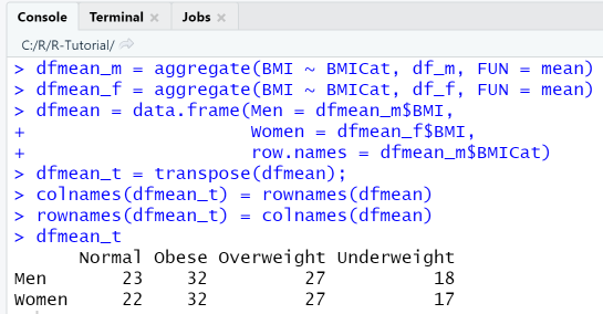
R packages and libraries

Top

R provides a large number of built-in packages, that are pre-installed, and a huge number of additional packages, that must be installed. The sheer number of packages can be confusing to R beginners, even more so, since you can choose between multiple packages that offer the same functionality. For example, plotting can be done with base R functions, with ggplot2, lattice or plotly. Depending on the requirements, one or the other package is better suited. For the start however, it is ok to stick with base R, the rest will come with practice and experience.

Tasks related to installation can be done in RStudio in the Packages-panel, also via the console using commands such as install(package). To check for the location of installed packages, you can use the command .libPaths(). Among the installed packages, the base-package contains all the R basic functions, arithmetic, input/output, basic programming support.

Among the contributed packages, two stand out: Tidyverse and the Shiny Web Application Framework. Tidyverse is a bundle of R packages for data science using an unified paradigm and language and providing functionality for data manipulation visualization. It serves the requirements of more advanced R applications: to be able to pre-process (aggregate and transform) and visualize data efficiently and on a high abstraction level. Shiny is a bundle of R packages representing a web application framework that enables to build reactive and responsive web applications.

ggplot2 (Tidyverse) Data Visualization
ggplot2 is a popular visualization package from the Tidyverse bundle, with its own grammar and plotting paradigm, and often used as replacement for the default R plotting functions. Plotting is done on a higher abstraction level, using the central function ggplot, specifying a data frame as source, adding so-called aesthestics and different layers. The example code conveys a first idea of how ggplot works: it simply creates a scatter plot of Height vs. Age using ggplot.

library(ggplot2)
age = c(rep(20, 10), rep(30, 5), rep(40, 5))
height = rnorm(20, mean=170, sd=5)
df = data.frame(Age = age, Height=height) # create data frame
ggplot(df, aes(x = Age)) + # create plot
  geom_point(aes(y = Height)) + # add point graph
  ggtitle("Scatterplot: Height vs. Age") # add title

dplyr (Tidyverse) Data Manipulation
dplyr provides functionality for data manipulation: subsetting, summarizing, rearranging, and joining data sets. You can filter rows with filter(), change the order or rows with arrange(), select columns with select(), etc. Additionally to the unified syntax, the strongest advantage is that you can perform these operations in a chain using the pipe-operator %>%. The example code conveys a first idea of how dplyr works: from the population data set we first filter all rows with BMI Category "Obese" and then select only the specified columns.

library(dplyr)
df %>% 
  filter(BMICat == "Obese") %>% 
  select(Age, Gender, Height, Weight, BMI)

data.table Data Manipulation
data.table is an R package that provides an enhanced version of data frames, with support for filtering, grouping, sorting in an SQL-like query syntax.

library(data.table)
age = c(rep(20, 10), rep(30, 5), rep(40, 5))
height = rnorm(20, mean=170, sd=5)
dt = data.table(Age = age, Height=height);dt
dt[, .(.N), by = .(Age)] # group by Age
table(dt$Age) # create frequency table for Age

Shiny Web Application Framework Web Application Framework
Shiny is a framework used to build interactive web applications with R. Its best features are automatic "reactive" binding between inputs and outputs and extensive prebuilt widgets. Shiny apps can be hosted in the cloud or used as a stand-alone display board and offer a wide range of applications. You can create Shiny projects and deploy them in the shiny.io cloud directly from RStudio.
For Shiny App examples, check out the Shiny Gallery and also the RVisLearner App developed for this tutorial, or the PredMaintApp demonstrating a decision tree classification for failure identification in a Predictive Maintenance use case.

Caret Supervised learning Regression Classification
The caret-package contains utility functions that support the model training process for supervised learning (regression and classification problems): (1) Preprocessing, (2) Data splitting, (3) Feature selection, (4) Training, (5) Model tuning. Example functions are createDataPartition() for splitting in train- and validation data, train() - sets up tuning parameters for a number of classification and regression routines, fits each model and calculates a resampling based performance measure, confusionMatrix() - calculates a cross-tabulation of observed and predicted classes with associated statistics.

Other useful R packages are ROCR, an R package for evaluating and visualizing classifier performance, and DT, an interface to the DataTables library, used in Shiny Apps.

R vs Python

Top

When starting to learn data science or planning a new data science project, a question often asked is, which language to choose: R, Python or yet another language or tool that has data science support (MATLAB, RapidMiner, ...). R and Python are the languages used most frequently for data science. R is a specialized language, somewhat preferred by statisticians and in academics, Python a general purpose programming language, somewhat preferred by computer scientists and in business.

Python being a general purpose programming language means that it is easier to learn and data analysis components are easier to integrate in software architectures. R being a specialized language means that the learning curve is slightly steeper, since part of its syntax, function names and design principles are specific to R. Both R and Python are fun and rewarding to work with, they can be used with Jupyter Notebook, and they can be integrated in visually pleasing web frontends.

Tools & References

This tutorial gives an introduction to R basic syntax. Starting here, there is much more to be learned and done: creating and validating regression and prediction models, advanced visualization using Tidyverse packages, etc.

You can test your basic understanding of R language syntax by taking the quizzes "R Fundamentals" and "R Functions".
For learning about data visualization with R, try out the RVisLearner, an interactive app build with R Shiny.

The R project: r-project.org/
The Comprehensive R Archive Network: cran.r-project.org/
An introduction to R: cran.r-project.org/doc/manuals/r-release/R-intro.html
Quick list of useful packages: support.rstudio.com/hc/en-us/articles/201057987-Quick-list-of-useful-R-packages
Tidyverse: R packages for data science: https://www.tidyverse.org/
R for Data Science: https://r4ds.had.co.nz/
DataCamp: Introduction to R: https://www.datacamp.com/courses/free-introduction-to-r