MATLAB Tutorial - An introduction for engineers
MathWorks' MATLAB is a commercial computing environment targeted at numerical computations and simulations. MATLAB offers functionality for creating and manipulating arrays and matrices, for plotting functions and data and for implementing mathematical algorithms that solve physical and engineering problems. This tutorial gives an introduction to the MATLAB environment and language as needed by engineers for learning Numerical Methods. Basic MATLAB syntax (variables, input, output, vectors, matrices, functions, plotting) is illustrated using example scripts.
Motivation
A computing platform like MATLAB offers a broad support for solving mathematical problems analytically as well as numerically. MATLAB functions and toolboxes hide implementation details and much of the underlying complexity. Engineers can set up models and generate solutions even without understanding the underlying numerical method very well initially, so they can just focus on their physical problem. Since powerful solvers are available, the focus is shifted from solving a problem to modeling it correctly.
MATLAB has powerful support for solving numerical problems that model engineering problems. For example, MATLAB's Ordinary Differential Equation solvers solve time-dependent problems with a variety of properties. The PDE (Partial Differential Equation) Toolbox provides functions for solving partial differential equations that model structural mechanics and heat transfer problems using finite element analysis. All functions are well-documented and there are many examples available.
Octave is an open source computing environment and scientific programming language that has the same basic capabilities as MATLAB. While the environment is not as sleek or user-friendly as MATLAB, it is free, and perfectly suited for learning MATLAB language basics. Most examples in this tutorial will also run in Octave.
Overview
The tutorial is structured in ten sections that explain usage of the MATLAB Integrated Development Environment and the most important MATLAB commands:
- 1 Install the environment
MATLAB IDE Octave IDE - 2 First lines in MATLAB
Commands clear clc Interactive mode Script mode Variables Comments - 3 Input and Output-Commands
disp fprintf input inputdlg Input from files - 4 Control flow
Conditional statements (if-else) Loops: for, while - 5 Vectors
Create vectors Vector operations Random numbers - 6 Matrices and arrays
6-1 Create matrices
6-2 Slicing matrices
6-3 Matrix concatenation
6-4 Matrix operations - 7 Tables: a spreadsheet-like data structure
Create tables Modify tables - 8 Functions
Global functions Local functions Anonymous functions - 9 Plotting in MATLAB
Line plot Subplot Figure and plot handle Surface plot Advanced plotting - 10 Symbolic computations
syms fplot diff int
1 Install the Environment
In order to run MATLAB scripts, a MATLAB installation is required. A test version can be downloaded from Mathworks website. Alternatively, you can download and install Octave, which is free. In the following we use the term integrated development environments (IDE) and refer to "MATLAB IDE" and "Octave IDE". After installation, the IDE's look similarly as in the screenshots below.
In MATLAB, the default window layout displays file browser, workspace, editor and command window
in a 4x4 grid, and be configured and aligned differently using the Layout menu.
In Octave, the default window layout organizes file browser, workspace and command history in the
left part of the main view and command window, documentation, editor and variable editor in the right part of the
main view. You can see either the command window or the editor, but not both at the same time,
which is an inconvenience. When running scripts, it is often required to see editor and output next to each other.
The only way to do this, is by undocking the command window, resizing it, and placing it on top of the main window.
MATLAB Environment
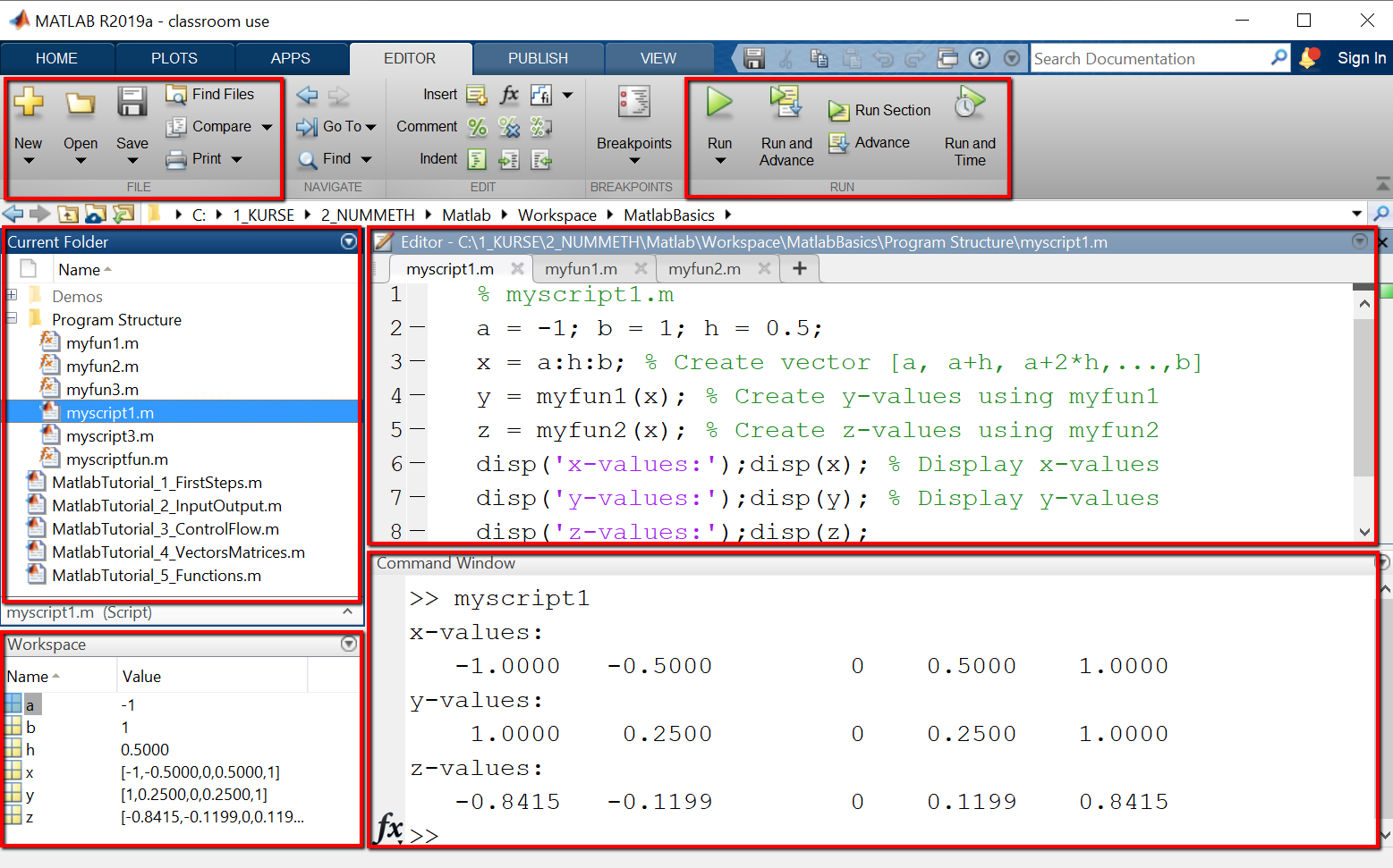
MATLAB's Editor-Tab is organized in four windows, that are used for developing and running scripts.
- File browser (top-left): displays the folders that contain m-files. Here you create new folders and new scripts.
- Workspace (bottom-left): displays the variables and functions of the running scripts.
- Editor (top-right): displays the contents of the script files. The actual programming is done in the editor.
- Command Window (bottom-right): displays commands and the output of statements.
Octave Environment
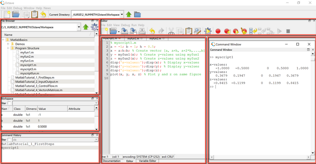
Octave IDE similarly is organized in five main windows, that are used for developing and running scripts.
- File Browser: displays the folders that contain m-files. Here you create new folders and new scripts.
- Workspace: displays the variables and functions of the running scripts.
- Command history: displays the history of commands. Can be cleared by using history -c.
- Editor: displays the contents of the script files. The actual programming is done in the editor.
- Command Window: displays commands and the output of statements.
A MATLAB program can be created in different ways:
- Interactive mode:
MATLAB can be used in interactive mode, by entering commands directly in the command window. Output is also shown in the command window. Interactive mode is useful for tutorials and for testing small program parts. -
MATLAB Script:
Larger MATLAB programs are collections of MATLAB scripts stored in a common folder. The folder can be anywhere on your computer but must be added to the MATLAB path by using HOME > Set Path Menu. - MATLAB LiveScript:
MATLAB LiveScripts are a special type of scripts with extended documentation features. While an .m-file contains source code and comments and displays output in the command window and figures in the figure editor, a LiveScript (.mlx file) offers more functionality. In a LiveScript, user input, source code and output including graphics are displayed in one single interactive window. The effect of a change in the source code can be seen directly and immediately in the output results (graphics, text output, etc.). While a pure code script is more efficient when the task is to solve a specific problem, MATLAB LiveScripts can be used as teaching tool and for demonstration purpose, since they convey a better understanding of the steps, commands and functions used to solve a problem.
A MATLAB script is a text file with the extension .m, that contains the statements and comments of the program.
MATLAB script names may contain only letters, numbers and subscript.
Valid names are for example myscript1.m, myscript2.m, myfun1.m, myfun2.m.
MATLAB scripts are created using the menu items in the EDITOR > FILE menu (New, Open, Save etc.)
and are executed using the menu items in the EDITOR > RUN-Menu (Run, Run and Advance, Run Section).
2 First Lines in MATLAB
| Top |
MATLAB statements are expressions or assignments, variable declarations , operations with variables, input- or output-instructions, control flow statements or function calls, that perform specific tasks (plots, mathematical computations etc.). MATLAB statements can be terminated with a semicolon or not. If terminated with a semicolon, a statement will not generate any output in the command window.
2-1 Commands for clearing, formatting, help
Before starting to explore the MATLAB language, we learn some commands that are needed frequently to keep a clean and organized workspace and command window.
- clear – Clears workspace variables. You can delete selected variables or all variables. Useful when you run multiple scripts that use the same variable names.
- clc – Clears command window (instructions and output). Useful when you want to start over with your script and do not need previously used commands or output.
- close all – Closes all open figures.
- format compact – Compactifies the command window output. More generally, the format command is used for formatting. For example format long changes the display of all floating point numbers in the command window to double precision. format short e is used for short scientific formatting.
- help – If you type help followed by the name of a command or function, the corresponding help page is displayed.
Example
Find out what the clc command does.
When typing "help clc" in the command window, the documentation for the clc command is shown as depicted. By clicking the displayed "Reference page ... "-link, the reference page for the command in the MATLAB online documentation is opened, with the complete information and examples on how to use the command.
Output

"Hello World" Program in MATLAB
A "Hello World" program is the smallest executable program in a programming language and prints the text "Hello World" to default output (here: the command window). We do it first in interactive mode and then in a script.
2-2 Interactive mode
| Top |
In interactive mode, we use only the command window. Statements are entered next to the command prompt (indicated by >>) and executed using ENTER.
Example
Using interactive mode and the command window.
Type the statement text='Hello World' in the command window and confirm with ENTER. As shown in the picture, the variable (here: text) and its content (here: Hello World) are shown as output in the command window. Next, type the statement disp('Hello World') and again confirm with ENTER. Again, the string is displayed, but this time without the name of the variable.
Output

2-3 Script mode
| Top |
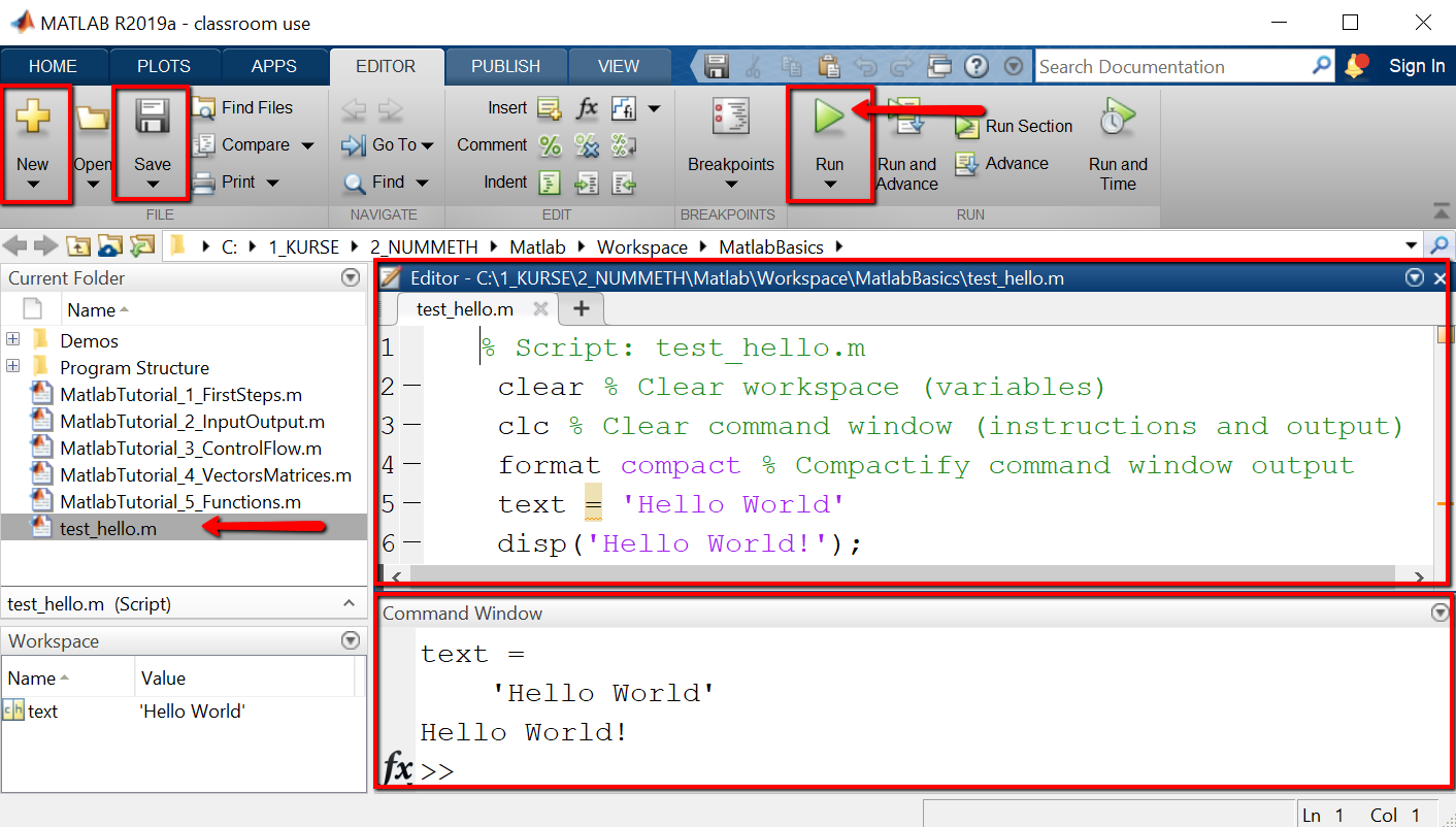
In script mode, we first create a new script with the name "test_hello.m", then type the MATLAB statements below in the script file and save it, and finally execute the script by clicking the "RUN"-Button.
Example
Using script files to store larger programs.
The code starts in line 1 with a comment (indicated by "%"-symbol), that states the name of the script file. Note that the following lines are also commented. In lines 2 and 3 we insert code for resetting / preparing workspace and command window. In line 4 we create a new variable "text" and assign it the value 'Hello world'. In line 5 we print the string 'Hello World' using disp().
% Script: test_hello.mclear;clc; % Clear workspace and command windowformat compact % Compactify command window outputtext = 'Hello World'disp('Hello World!');
Output
The MATLAB platform after creating, editing, saving and running the script test_hello.m looks as shown. In the menu bar we have highlighted the New, Save and Run menu items, that have been used to create the new script, save, and execute it in turn. Top-right displays the editor with the code of the script test_hello.m and bottom-right the command window with the output after executing the script.
2-4 Comments in MATLAB
| Top |
Comments in MATLAB start with a "%"-symbol followed by text. Comments are used for documentation purpose, they are not executed by the system. Two percent-symbols "%%" mark a section. Sections can be executed separately using the RUN SECTION-Button.
%% Section 1% Comment 1: This is the first comment for section 1.text = 'Let''s start simple' % Here we assign a value to the variable named text%% Section 2% Comment 2: This is the first comment for section 2.a = 10 % Here we assign a value to variable ab = 20 % Here we assign a value to variable b
2-5 Variables and data types
Variables are named memory spaces that store the data of your program. MATLAB variables are declared by simply assigning a value to them. The data type (number, string, array etc.) is assigned automatically by MATLAB. For example, all numbers (integer, floating points) are stored internally as double precision floating point numbers. Knowing the data type is important, since the data type determines the set of operations that you can perform with your variables. For example, you can add two numbers or concatenate two strings with the "+"-operation as in the example below, but it is not possible to add a number to a string: sum = a + " apples" is an invalid statement. Before appending a number to a string, it must be converted to a string using num2string: sum = num2string(a) + " apples" is a valid statement.
Example
Using variables: declaration and operations
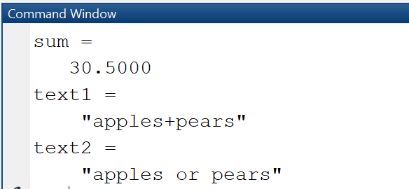
The example shows how to declare variables (numerical and string) and perform operations on them. Note that the +-symbol denotes different operations: in line 3, the addition of numbers, in line 5, the concatenation of strings.
% test_variables.ma = 10; b = 20.5;sum = a + bs1 = "apples";s2 = "pears";text1 = s1 + "+" + s2text2 = replace(text1, '+',' or ')
Output
When executing the script test_variables.m, output in command window is as shown.
Code explanation:
- Line 2: Declare two variables a, b by assigning values to them. Since the declarations are terminated with semicolon, output of the variables to the command window is suppressed.
- Line 3: Add the two variables (actually, their values) and store the result in the variable sum.
- Line 4: Declare two string variables s1, s2.
- Line 5: Concatenate the strings to form a new string.
- Line 6: Replace the "+"-character with the string ' or '.
Data types
MATLAB supports different data types, that are represented by classes:
- Numerical data types: int, single, double
- Boolean data types: logical
- String data types: string, char
In order to find out the exact data type and size of your variables, use the commands whos, class. With whos, you can find out size and type of workspace objects. With class, you can find out the data type of a variable.
Example
Declare variables and find out their data type.
We declare two variables a and b by assigning numeric values, 10 and 20.5 respectively. Then show information about them using whos.
a = 10;b = 20.5;whos awhos b
Output

MATLAB assumes the data type of a variable to be double even when you assign an integer number and accordingly reserves 8 Byte of space. Also, a variable is considered to be matrix with one row and one column, this is why the size is shown as 1x1.
String variables
String variables in MATLAB can be either of class "string" or of class "character array". When you create a string using single quotes, it is stored as character array. When you create a string using double quotes, it is stored as a string. A character array is a sequence of characters, just as a numeric array is a sequence of numbers. The String class provide a set of functions for working with text as data.
Example
Declare string variables and find out their data type.
text1 = "Hello"whos text1text2 = 'from Kaiserslautern'whos text2
Output

3 Input and Output-Commands
| Top |
Data stored in variables can either be viewed in the workspace or displayed in the command window. While the workspace shows the raw variable values, the command window is used for formatted output.
3-1 Output to command window
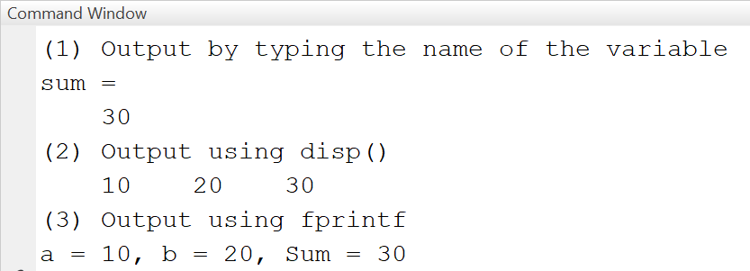
There are three ways to output variable values to command window.
- Type the name of a variable in a new line, with no terminating semicolon. In an assignment statement, omit semicolon at the end of a statement. The content of the variable then is displayed in the command window.
- Use disp()-function. This function takes as argument a variable / vector / matrix and displays it, omitting the name of the variable.
- Use fprintf()-function. This function builds a formatted output by using placeholders for the variables to be inserted. In our example, the value of variable a will be inserted in the place indicated by the first "%d", the value of variable b will be inserted in the place indicated by the second "%d" etc.
Example: Output to command window
Different ways to create output to command window.
In this example we calculate the sum of two variables and generate output in the command window.
% test_output.ma = 10; b = 20; sum = a + b;% (1) No semicolondisp('(1) Output by typing variable name')sum % output: sum = 30% (2) Use dispdisp('(2) Output using disp()')disp([a b sum]) % output: 10 20 30% (3) Use fprintf for formatted outputdisp('(3) Output using fprintf')% output: a = 10, b = 20, Sum = 30fprintf('a = %d, b = %d, Sum = %d\n', a, b, sum)
Output
When running the script test_output.m, output looks as displayed.
3-2 Input with input()
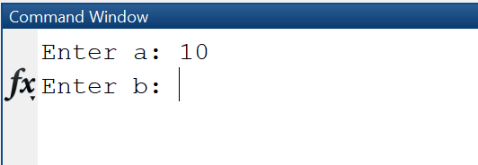
When presenting a MATLAB script to non-technical users, it may be helpful to let them enter configuration parameters as input from the command window or an input dialog. Input entered in the command window can be stored in variables using the input()-function.
Example
Input using prompt.
% Display a prompting textprompt = 'Enter a: ';% Read inputa = input(prompt);prompt = 'Enter b: ';b = input(prompt);sum = a + b;fprintf("Sum = %.2f\n", sum);
Output
Input dialog
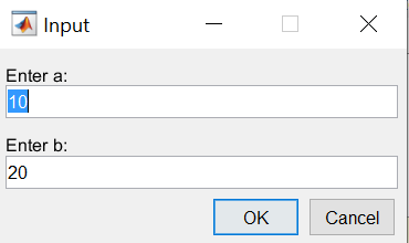
An input dialog as shown below is created using the MATLAB-function inputdlg. We pass four arguments to the function:
- prompt -- the labels of the input fields
- dlgtitle -- the title of the dialog
- windowsize -- the size of the window
- definput -- specifies the default value for each edit field. The definput argument must contain the same number of elements as prompt.
The function returns an array of strings "answer", that contains the values entered in the edit fields.
Example
Input dialog for two variables.
prompt = {'Enter a:', 'Enter b:'};dlgtitle = 'Input';windowsize = [1 50];definput = {'10','20'};answer = inputdlg(prompt, dlgtitle, windowsize, definput)a = str2num(answer{1})b = str2num(answer{2})
Output
3-3 Input from files
Many applications require to read tabular data from *.txt, *.csv or *.xlsx files, or binary data (images). For this type of requirement, MATLAB offers functions such as inputdata, readtable and load. They all require as input a file, specified by its name including the path, and return an internal representation of the data, either as table or as struct or array. If only the filename is specified, MATLAB searches for a file in the same folder where the script is placed. Alternatively, it is possible to specify the full path to the file, for example 'C:\temp\accidents.csv'. Note that when importing from Excel, the row and column headers should be specified correctly. Also, it is important to use the correct delimiters for the decimal point, in a computer with German settings, this will be comma (,), else dot (.).
- A = importdata(filename, delimiter) loads data into array A. This function is used for importing tabular data as well as images.
- T = readtable(filename, options) reads tabular data from a file and stores it internally in a table object. This function is useful when you have spreadsheet-like data as in an excel-sheet, where each column has its own data type. Column headers are imported (or not) by specifying the options 'ReadVariableNames' and 'PreserveVariableNames'.
- T = load(filename) loads variables or data from a file into workspace: if the file is a *.mat-file, then in loads the variables from this file, else if it is a text-file, it loads the data into a double-precision array.
When developing a numerical method, it is often required to convert the table object returned by importdata into an array or extract single columns or rows of the imported table into a column vector. This is done by using the function table2array as in the next example.
Example: Importing data from files
Using importdata, readtable and load
For this example we use two input files, accidents_5.csv and accidents_5.xlsx, that we store in the same folder as our test script. The csv-file contains number-only entries separated with semicolon and has no headers. The Excel-file contains the same data as the csv-file, but with headers.
%% Load data using importdata% (1) Load data using importdataA1 = importdata('accidents_5.csv', ';')% (2) Alternatively: Use readtableT = readtable('accidents_5.xlsx', 'ReadVariableNames', true)% Convert the table into an arrayA = table2array(T(2:end, 1:end))% Extract the second rowrow2 = A(2,:)% (3) Alternatively: Use loadA2 = load('accidents_5.csv')%% Find out the type of the returned objectswhos T % It's a tablewhos A1 % It's an arraywhos A2 % It's an array
Output in the command window
The import stores data as array or table objects
 A1 =
            1      493782         164
            2      572059          43
            3      608827          98
            4      626932         101
            5      642200         100
 T =
   5×3 table
     Nr    Population    Accidents
     __    __________    _________
     1     4.9378e+05       164
     2     5.7206e+05        43
     3     6.0883e+05        98
     4     6.2693e+05       101
     5      6.422e+05       100
 A =
            2      572059          43
            3      608827          98
            4      626932         101
            5      642200         100
 row2 =
            3      608827          98
 A2 =
            1      493782         164
            2      572059          43
            3      608827          98
            4      626932         101
            5      642200         100
4 Control flow
| Top |
Control flow statements are used to determine which block of code to execute at run time (conditional statements, if-else) or to execute a block of code repeatedly (while-loop, for-loop). In MATLAB, these multiline statements are terminated using the keyword end.
4-1 Conditional statements
Conditional statements are used to control which of two or more statement blocks are executed depending on a condition. In MATLAB, as in most programming languages, they are implemented using the if-else-syntax. The condition after the if or elsif-keyword can be enclosed in round brackets, this is optional.
Switch-case statements execute one of many different cases based on the evaluation of a variable. Switch-case can be used for performing a specific task according to user input. Different from C, Java or other programming languages, in MATLAB it is not required or allowed to terminate a case with break.
Example 1: If-else
Show message according to the size of the number
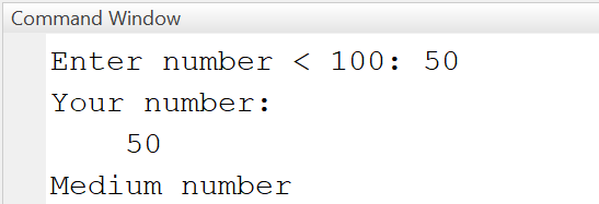
In this example the user is asked to enter a number smaller that 100 and according to the size of the input a message is displayed. In line 5, the condition "a < 30" is evaluated: If true, the statement in line 5 is executed and the program flow continues in the first line after the if-else-statement.
% test_ifelse.mprompt = 'Enter number < 100: ';a = input(prompt);disp('Your number:'); disp(a); % display itif a < 30disp('Small number!')elseif a < 80disp('Medium number!')elsedisp('Large number!')end
Output
Example 2: Switch-case
Execute different tasks depending on user input
If user input equals A, execute addition, if B, subtraction, if C, multiplication, (and so on) otherwise display an appropriate message.
prompt = "Choose action: A=add, B=sub, C=mult: ";text = input(prompt, "s");a = 10; b = 20;switch textcase 'A'result = a + bcase 'B'result = a - bcase 'C'result = a * botherwisedisp('Invalid operation')enddisp("Done!")
4-2 Loops
Loops are used for program flow control, so that statements can be executed repeatedly, as long as an execution condition is met. MATLAB has two loop commands: while loop and for loop. For additional control of the loop execution, the commands break and continue are used: break allows you to exit a loop if a given condition is fulfilled, with continue you can skip loop steps depending on a condition.
For-loops have a more compact syntax and are used frequently when working with tables and matrices. While-loops are used when more general loop conditions apply, for example input validation: as long as an user does not enter a required input format, he is asked to repeat his input.
While Loop
A while loop allows statements to be executed repeatedly, as long as an execution condition is met. The variable that is queried in the condition must be explicitly incremented in the body of the loop. If there is no increase in the variable, the loop is executed endlessly.
Example 1: While-Loop
Calculate sum 1+2+3+4+5
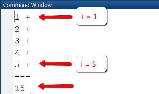
In this example, we calculate the sum of first n numbers, 1+2+...+n. First, the variable s that will store the sum is initialized with 0. A counting variable i is initialized with 1. In line 3 the loop condition "i <= n" is checked. If "true", the statements in line 4-6 are executed (print the value of i, add the value of i to the value of sum, increment the value of i) and then the loop condition is checked again and the loop is repeated.
n = 5; s = 0;i = 1; % (1) Initialize counter iwhile i <= n % (2) Check conditionfprintf("%d + \n", i);s = s + i;i = i+1; % (3) Increment counterendfprintf("---\n");fprintf("%d\n", s);
Output
While-loops that use a counting variable can be written more concisely as for-loop.
Example 2: While-Loop
Calculate sum 1+3+5+7+9
The next example calculates the sum of uneven numbers less than a given n.
n = 10; s = 0;i = 1;while i <= ns = s + i;i = i + 2; % Increment counter by 2endfprintf("s = %d\n", s) % Output: s = 25
Example 3: While-Loop
Infinite loop with break
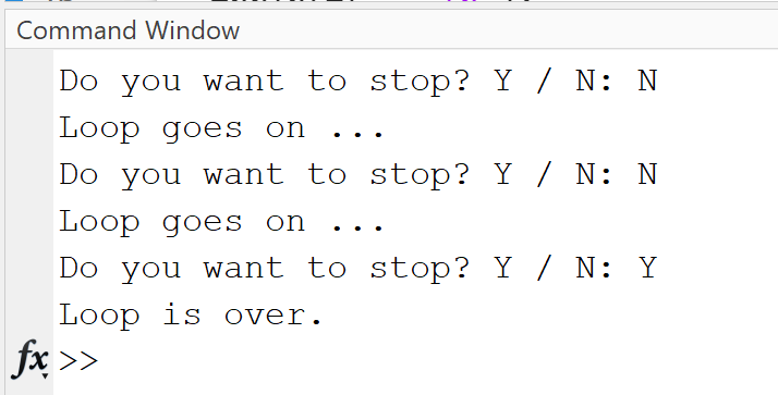
In this example, the user is asked to confirm if a loop should be continued or stopped. In line 1, the infinite loop is started using while 1. Since 1 is evaluated as true, the statements in the loop will be executed endlessly, unless a break is inserted, that allows to exit the loop.
while 1txt = input("Do you want to stop? Y / N: ", "s");if txt == "Y"break;elsedisp("Loop goes on ...")endenddisp("Loop is over.")
Output
For Loop
A for loop is a counting loop that defines a start and end condition for a counting variable (loop counter) and repeats a statement or a group of statements for a number of loop passes as specified by the loop counter. The loop counter is increased by 1 (or another step size) after each loop pass.
Example 1: For loop
Calculate sum 1+3+...
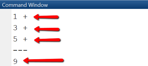
The sum of odd numbers smaller than n: sum = 1+3+..., is calculated here using a for loop. The for loop uses a counter variable i to control how often the statements in the loop are executed. In this example it starts at index 1, uses step size 1 and ends at index n.
n = 6; s = 0;% Start at index 1, use increment 2, end at index nfor i=1:2:nfprintf("%d + \n", i);s = s + i;endfprintf("---\n");fprintf("%d\n", s);
Output
Example 2: Nested for loop
Create 3x3 identity matrix
Nested loops are needed a lot when solving problems that involve matrix computations. The usage of for- instead of while-loop is preferred if you nest loops, since the syntax is more compact and there are clear counting variables: row index for the outer loop and column index for the inner loop. In this example, we use two nested for-loops to create the 3x3 identity matrix. MATLAB's eye function does exactly the same thing, it creates the identity matrix in just one line.
# Create 3x3 identity matrixm = 3; n = 3;for row=1:mfor col = 1:nif row == cola(row,col) = 1;elsea(row,col) = 0;endendend# Create identity matrix using eyea = eye(3)
MATLAB provides high-level functions for many cases where otherwise a loop would be needed.
You can calculate sums and means of vectors or matrices using MATLAB's sum and mean functions,
in just one line, as the following example code shows.
% Calculate sum of first 5 numberss = sum(1:5) % Output: 15% Calculate sum of the elements of a given arraya = [10, 20, 50, 5, 5, 50]s = sum(a) % Output: 140% Calculate mean value of the elements of as = mean(a)
This means that in MATLAB loops are used less than you would have to in other programming languages. Loops are still needed when implementing non-standard tasks, such as task-specific input validation or solvers.
5 Vectors
| Top |
Vectors are one-dimensional arrays that store data of the same data type (numerical or strings). Matlab vectors can be stored in row or column format.
For example, x = [1 4 9] will be a row vector, and x = [1; 4; 9] will be a column vector.
Elements of a vector are accessed using an index that starts at 1.
For example, to access element i in vector x, we write x(i).
Create vectors
Vectors are created in different ways: by listing their elements explicitly in square brackets, using special MATLAB functions such aus zeros(), ones(), linspace() or using for-loops.
Example: Vectors
Create vector with 5 elements
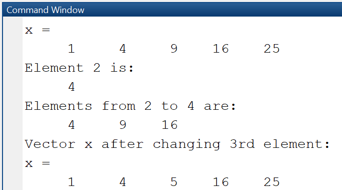
We first create a row vector with 5 elements, display the second element of the vector, then the elements 2, 3 and 4 and change element 3 to be the sum of the first two elements.
x = [1 4 9 16 25]disp('Element 2 is: ')disp(x(2))disp('Elements from 2 to 4 are:')disp(x(2:4))% Change element 3 to be sum of element 1 and 2disp('Vector x after changing 3rd element:')x(3) = x(1) + x(2)
Output
Example: Vectors
Find out size and length of vector
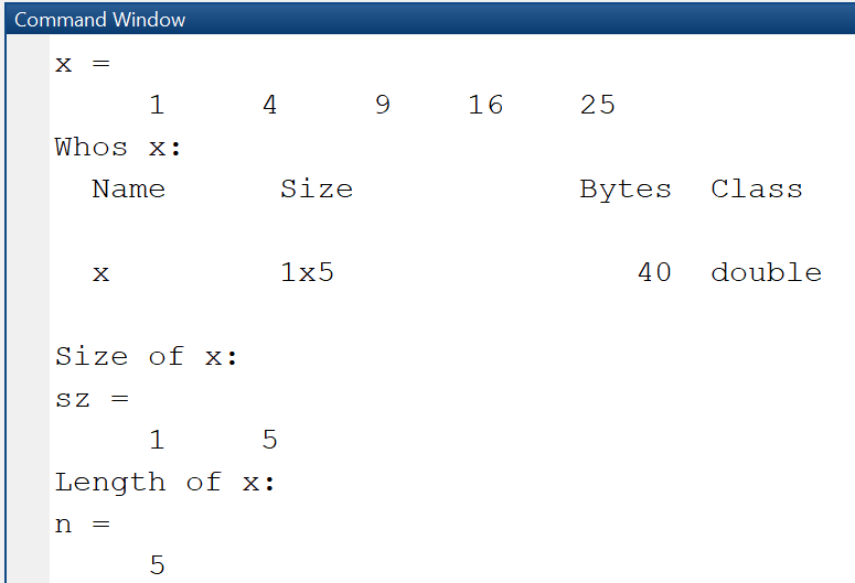
Using the whos command, we can see that the vector x is actually a matrix with 1 row and 5 columns, is of class double and uses 40 bytes of storage.
x = [1 4 9 16 25]disp('Whos x:')whos xdisp('Size of x:')sz = size(x)disp('Length of x:')n = length(x)
Output
Random numbers
An important usecase for creating vectors is that of generating pseudo-random numbers. This can be done using the functions rand, randi, randn. rand creates uniformly distributed random numbers of data type double, by default in the interval (0,1), and depending on the provided arguments, you can generate a matrix, a column or row vector, or a single number. randi creates uniformly distributed random integers, as matrix, column or row vector.
Example: Random numbers
Using rand and randi
% Create 3x5 matrix; random numbers in (0, 1)r_mat = rand(3, 5)% Col vector with 5 random elements in (0, 1)r_col = rand(5, 1)% Row vector with 5 random elements in (0, 1)r_row = rand(1, 5)% Row vector with 5 elements in range (a, b)a = 10;b = 20;r_row_10_20 = rand(1, 5)*(b-a) + a% Create n integer random numbers in [a, b]a = 10;b = 20; n = 5;r_int_10_20 = randi([a, b],1, n)
Output

Vector operations
MATLAB supports vector operations of two kinds: mathematical operations according to the rules of
linear algebra (transposition, addition, multiplication) and array-type elementwise operations.
Elementwise operations are distinguished from vector operations by usage of the dot operator (.).
x * y means matrix multiplication, and works only if x is a 1xn row vector and y is a nx1 column vector.
x .* y means elementwise multiplication and works only if x and y are both row (or column) vectors of same size.
Vector and elementwise operations are the same for addition and subtraction, so the operators .+ and .- are not used. Since vectors actually are a special type of matrix, these operations are the same as the described below for matrices.
Example: Vector operations
Create vector with 5 elements
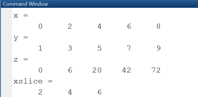
We first create a row vector x with 5 elements, then a row vector y from x by adding 1 to each element, and a third vector z by elementwise multiplication of x and y.
x = 0:2:8 % x = 0,2,4,6,8% Add 1 to each elementy = x + 1 % y = 1,3,5,7,9% Multiply x and y elementwisez = x .* y % z = 0*1+2*3+...+8*9% Slicing% Extract a slice from 2 to 5xslice = x(2:4) % x1 = 2,4,6
Output
6 Matrices
| Top |
MATLAB scripts store their data in one- and multi-dimensional arrays (e.g. vectors, matrices) if the elements are of same data type, in cell arrays that may contain elements of varying types and sizes, or in tables, if the elements are spreadsheet-like with columns of same data type. Each of these data structures support their specific set of operations and special functions for manipulating the data.
Elements of a matrix are accessed using a row index and a column index that both start at 1. For example, to access element in row i and column j in a matrix A with m rows and n columns, we write A(i, j). Element with row-index 1 and column-index 1 is accessed with A(1, 1), etc.
6-1 Create matrices
Matrices are created in different ways: by enumerating their elements explicitly in square brackets, by pre-allocating them with default values using functions such as zeros() or ones(), or using for-loops. Sometimes it is useful to start with an empty matrix and later append rows and columns. An empty matrix A can be created with the command A = [].
Create matrix using enumeration
When declaring a matrix by explicit enumeration, row elements are separated by a space and columns are separated by semicolon.
Example: Create matrix
Create matrix by enumeration
In this example we declare a matrix with two rows and three columns, display it using disp, and find out type and size using whos. The whos-command shows that it is indeed a 2x3 matrix and uses up 48 bytes of memory.
A = [1, 2, 3;4, 5, 6]; % 2 rows, 3 colsdisp('Matrix A:')disp(A)whos A
Output

Create matrix using functions
Many mathematical problems require to use matrices initialized with specific values, such as the identity matrix.
In MATLAB, the declaration of these matrices is done using MATLAB functions such as
zeros - initializes a matrix with all zeros, ones - initializes a matrix with all ones,
rand - creates a matrix with random values,
or eye - creates the identity matrix.
Example: Create matrix
Create matrices using functions zeros, ones, eye
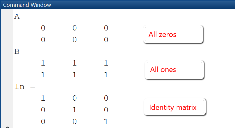
In this example we create three matrices: A is a matrix with m rows and n columns whose elements are initialized with zeros. B is a mxn matrix whose elements are all initialized with 1. I_n is the identity matrix with n rows and n columns, with ones on the diagonal and 0 on all other elements.
m = 2; n = 3;% mxn matrix with elements initialized to 0A = zeros(m, n)% mxn matrix with elements initialized to 1B = ones(m, n)% nxn identity matrix with 1 on diagonalI_n = eye(n, n)
Output
Create matrix using for loops
The creation of a matrix using for loops is required when the size and even the element values change dynamically
depending on some parameters. In this case, it is recommended to preallocate the maximal required memory using the zeros()-function.
m = 3; n = 4; % m rows and n columnsA = zeros(m, n); % create a mxn matrix initialized with zerosfor i=1:m % loop over the rowsfor j=1:n % loop over the columnsA(i,j) = i*j; %endenddisp(A)
6-2 Slicing matrices
Accessing elements from a matrix is done using indexing and slicing.
With indexing, we access single elements, for example A(2,3).
With slicing, we access selected rows and columns, specified either as a list or range of indexes.
For example, in a matrix A with 5 rows and 3 columns, the expression A([1, 3, 5], :) will return
rows 1, 3 and 5 and all columns. The colon indicates that all rows are extracted.
The expression A(2:4, [1, 3]) will return the rows from 2 to 4 and the columns 1 and 3.
Example: Slicing matrices
Extract elements from a matrix
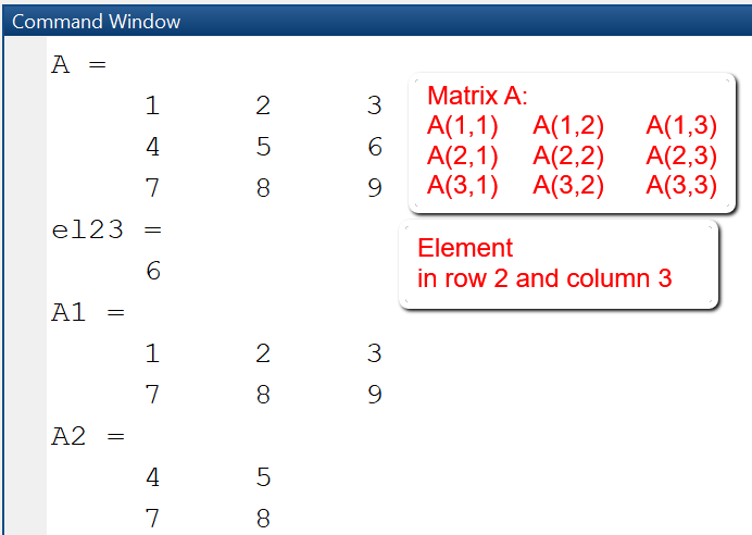
In this example we first extract the element with row-index 2 and column-index 3 and store it in a variable el23. Then we extract rows 1 and 3 and all columns and store the result in a new matrix A1, finally we extract the rows from 2 to 3 and columns from 1 to 2 and store the result in a new matrix A2.
A = [1, 2, 3; 4, 5, 6; 7, 8, 9]el23 = A(2,3) % el23 = 6:% Extract rows 1 and 3A1 = A([1,3],:) % A1 = [1, 2, 3; 7, 8, 9]% Extract rows 2 and 3 and and columns 1 and 2A2 = A(2:3,1:2) % A2 = [4, 5; 7, 8]% Extract rows 2 to end and and columns 1 to endA2 = A(2:end,1:end-1) % A2 = [4, 5; 7, 8]
Output
6-3 Matrix concatenation
Matrix concatenation is used to create a new matrix by joining existing matrices with matching dimensions.
Vertical concatenation is possible when you have two matrices A1 and A2 with the same number of columns.
Then by writing [A1; A2], you get a new matrix in which the rows of A2 have been appended to the rows of A1.
Horizontal concatenation is possible when you have two matrices A1 and A2 with the same number of rows.
Then by writing [A1, A2], you get a new matrix in which the columns of A2 have been appended to the columns of A1.
Example: Concatenate matrices
Add rows and columns to a matrix
A special case of concatenation is appending new rows or new columns to a matrix.
A = [1 2 3; 4 5 6]row = [7 8 9]col = [10; 11]% Append row to A% Concatenate A and row verticallyA1 = [A; row]% Append column to A% Concatenate A and col horizontallyA2 = [A, col]
Output
 A =
     1     2     3
     4     5     6
 row =
     7     8     9
 col =
    10
    11
 A1 =
     1     2     3
     4     5     6
     7     8     9
 A2 =
     1     2     3    10
     4     5     6    11
6-4 Matrix operations
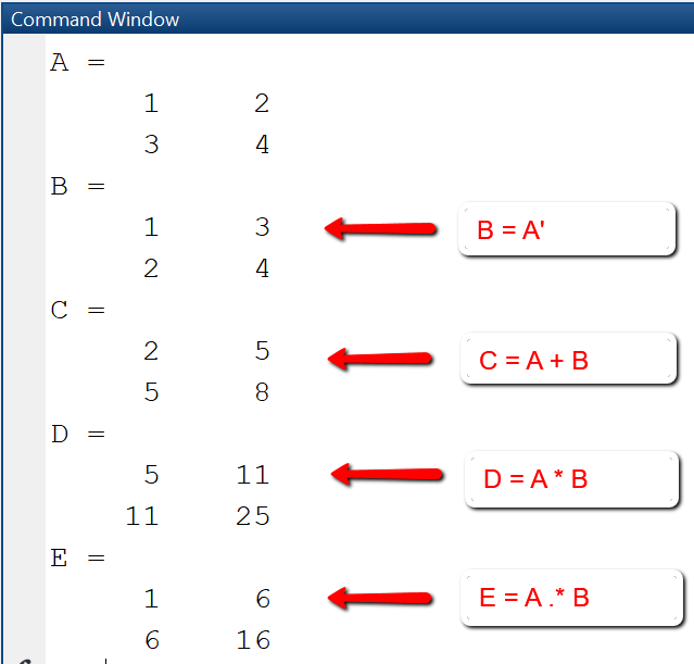
MATLAB supports matrix operations of two kinds: mathematical operations according to the rules of linear algebra (transposition, addition, multiplication) and array-type elementwise operations. Elementwise operations are distinguished from matrix operations by usage of the dot operator (.): A * B means matrix multiplication, A .* B means elementwise multiplication, A.^2 means that each element of the matrix is taken at power 2, etc. Since matrix and elementwise operations are the same for addition and subtraction, the operators .+ and .- are not used.
Example: Matrix operations
This example shows frequently used matrix operations: transposition, addition, multiplication and elementwise multiplication. The transposed of a matrix A is obtained by writing A', i.e. the matrix name followed by a quotation mark.
% Transpose a matrixA = [1 2; 3 4]B = A' % B = [1 3; 2 4]% Matrix additionA = [1 2; 3 4];B = [1 3; 2 4];C = A + B % C = [2 5; 5 8]% Matrix multiplicationA = [1 2; 3 4];B = [1 3; 2 4];D = A * B % D = [5 11; 11 25]% Elementwise multiplicationA = [1 2; 3 4];B = [1 3; 2 4];E = A .* B % E = [1 6; 6 16]
Output
7 Tables
| Top |
MATLAB tables are data structures used for storing and manipulating spreadsheet-like data, with named columns ("variables") and possibly row names. Different columns may have different data types, but the elements of one column must have the same data type. Elements can be accessed via their index as well as via row and column names. The table data type is used mainly for statistical tasks, for example, when you need to evaluate statistical properties (mean, standard deviation, min, max) of the variables. Tables are also useful for creating nice tabular representations of data obtained from measurements or from testing a numerical method.
Tables are created from column vectors using the table()-function with different arguments, from matrices using the function array2table(), or by importing data from a spreadsheet or csv-file using readtable(). The properties of a table T such as DimensionNames, VariableNames, RowNames can be found out and set by using the T.Properties-syntax, as shown in the following examples.
Create tables from column vectors
One way to create a table is to use already existing vectors, which must be column vectors and must have the same number of elements. The table created in this way will automatically have the name of the vectors as column names.
Example 1: Create table from column vectors
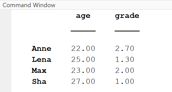
In this example, we create a table from the column vectors age and grade and specify the vector student as row names.
% Create a table from existing columns vectorsstudent = ["Anne", "Lena", "Max", "Sha"]';age = [22, 25, 23, 27]';grade = [2.7, 1.3, 2.0, 1.0]';T_stud = table(age, grade);% Add row namesT_stud.Properties.RowNames = student;T_stud
Example 1: Create table from column vectors
Output
Modify tables
Tables can be modified in various ways: you can add / remove / replace rows or columns, extract data, calculate statistical values for the table's variables (columns), plot the the table's variables..
Example 2: Append row with statistical values
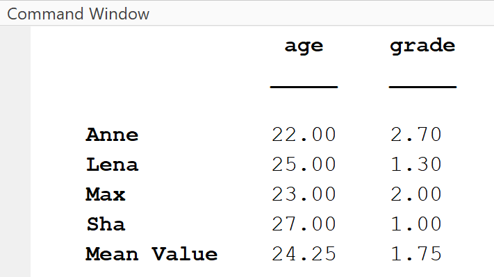
Next, a row is created that contains the mean values of the age and grade columns, and subsequently appended to the table.
% Calculate row with statistical valuesrow = table(mean(T_stud.age), mean(T_stud.grade));row.Properties.VariableNames = ["age", "grade"];row.Properties.RowNames = ["Mean Value"]';% Append row to tableT_stud = [T_stud; row]% (4) Extract single row: here: Anne's dataanne = T_stud('Anne', :);
Example 2: Append row with statistical values
Output
8 Functions
| Top |
A function is a reusable piece of code that is executed only when called. It is defined once and can be called multiple times.
Functions may have parameters and also may return parameters. The most frequent application of functions is to use predefined MATLAB-functions such as plot (for plotting) or linspace for creating equidistant vectors, or solvers such as ode45.
However, when writing larger MATLAB programs, you should structure them using self-defined functions, or, in a more advanced setting, object-oriented programming and classes.
User-defined functions can be defined in multiple ways:
- Global function: Function is stored in a separate m-file.
- Local function: Function is stored inline in the script where it is called.
- Anonymous function: Function is defined as an anonymous function in the script where it is called.
Important: While the variables of a MATLAB script are displayed in the workspace, the variables used in a function are local variables and not visible in the workspace. Global functions must have an unique name, must be on the MATLAB path and can be used in any other script. Local and anonymous functions are visible only in the script in which they have been defined, their name must be unique within the file in which they have been defined.
(1) Function stored in a separate m-file
In most cases, it is recommended to put the code of a function in its own function script. A function script is a MATLAB m-file that contains only the definition of a single function and cannot be executed as a "normal" script. Function and function script must have the same name, for example a function with name myfun1 must be stored in a function script with name myfun1.m. By storing a function in its own script, the function can be used by any other script in the MATLAB path by calling it with specific arguments.
Defining a function
Functions begin with the keyword "function", followed by the statement
outputargs = function_name(inputargs)
and end with the keyword "end". The actual function statements that define the relationship between the input arguments and the
output arguments are written in the function body between the first line and the last line.
In order to display the general syntax of a function definition and generate a template for a new function, we use the
New > Function-Button in the EDITOR-Tab. This creates a new function script "untitled.m" for the function "untitled" with two
generic input arguments and two generic output arguments.
Starting with this template, we create our own functions by changing name, arguments and code as needed.
function [outputArg1,outputArg2] = untitled(inputArg1,inputArg2)%UNTITLED Summary of this function goes here% Detailed explanation goes hereoutputArg1 = inputArg1;outputArg2 = inputArg2;end
Example: Functions
Define and call a function myfun1.
In this example, we create a function myfun1 that takes as input an array-parameter x and calculates the function values y = x*exp(-x2). The code to the left shows the function definition in the function script. In the test script myscript1.m we first create an equidistant vector x, then calculate the y-values by calling the function myfun1 and finally create a plot of the so created x,y-values.
Function myfun1.m
function y = myfun1(x)% Define the function y = x exp(-x^2)% Input: x -- a vector% Output: y -- a vector (same size as x)y = x .* exp(-x.^2);end
Script myscript1.m
x = -5:0.1:5; % Create vector xy = myfun1(x); % Calculate yplot (x, y, '+-'); % Plot y vs. xtitle('y(x) = x * exp(-x^2)');xlabel('x'); ylabel('y');
Output
MATLAB's plot-function is used to create 2D-line plots of data given as (x,y)-values. The plot-function takes as input two vectors that must be of same size, plus a number of formatting options for specifying line type, color, width, title, legend, axis labes etc.
(2) Local functions
Functions that will be used only in one script can be stored as local functions inline in that script, and should be placed at the end of the script. Local functions are visible only in the script in which they have been defined and cannot be used in other functions. Why use local functions at all, since the primary goal of a function is to make it reusable? There are situations when you develop new solvers for numerical methods and program variants of the same function, so you need to use it only locally in a test setting and also want to reuse the function name.
Example: Local functions
Define and plot two functions
In this example, we create two functions myfun1 and myfun2 inline in the test script "test_localfunction.m". Both functions myfun1 and myfun2 have as input parameter a vector x, and calculate the y-values for given mathematical functions.
% test_localfunction.mx = -1:0.1:1;plot(x, myfun1(x), '+-');hold onplot(x, myfun2(x), '+-');legend('myfun1','myfun2');title('Line-plot of two functions');xlabel('x'); ylabel('y');function y = myfun1(x)y = sin(x) .* exp(-x.^2);endfunction y = myfun2(x)y = cos(x) .* exp(-x.^2);end
Output
In line 4 we used the command hold on so that MATLAB displays both plots on the same figure.
(3) Anonymous functions
An anonymous function is a function that is not stored in a script file, instead it is associated with a variable of type function_handle.
Informally, it is an inline function that is written in just one line with the help of the @-symbol.
Anonymous functions are used for functions whose defining statement can be written in just one line.
General syntax is <function_name> = @ (<param_list>) ( <computation>).
Example: Use anonymous functions
In this example three mathematical functions are defined as anonymous functions.
- Line 1-3: Define function f(x) = sin(2πx) and then calculate the function values at points x = 1 and x = 2.
- Line 4-8: Define polynomial p(x) = 1 + 2x + x2 and then calculate the function values at the equidistant points x = [0, 0.5, 1.0, 1.5, 2.0]. Since in the definition of the polynomial the dot-operator is used, it is allowed to pass a vector as argument to the function.
- Line 8-11: Define a function of two variables u(x,y) = 25xy, where x and y are allowed to be vectors of same size. Then, create two vectors x, y using linspace and calculate the function values z for these vector arguments.
% Example 1: Sin-Functionf = @(x) sin(2*pi*x);y1 = f(1); y2 = f(2);% Example 2: Polynomialp = @(x) (1 + 2.*x + x.^2);x = 0:0.5:2; % x = [0, 0.5, 1.0, 1.5, 2.0]y = p(x);% Example 3: Function with two variablesu = @(x,y)(25.*x.*y);x = linspace(0,1,10); y = linspace(0,2,10);z = u(x, y);
9 Plotting in MATLAB
| Top |
When solving a mathematical problem such as an ordinary or partial differential equation numerically, it is important to be able to visualize the solution and the intermediate steps easily, as this helps the intuitive understanding of the physical problem. MATLAB supports graphics and plotting via number of functions for creating different types of line plots (plot, area), statistical plots: (histogram, boxchart, scatter), surface and mesh plots (surf, mesh, contour, quiver).
MATLAB plots are organized in figures and created with the figure command. The figure-command allows to specify options for the creation of the figure window, such as position and title. If the command figure is not specified, a figure is created by default.
9-1 Line plots with plot
The simplest plot is the line plot of a function y = f(x), using the function plot(). The plot-function has the general syntax plot(X,Y), that creates a line plot of the data in Y versus the corresponding coordinate values in X. X and Y must be vectors or matrices with matching size. For example, in order to create a plot of y = f(x) = x^2 for the discrete values X = [1,2,3,4,5] and Y = [1,4,9,16,25], we write
plot([1,2,3,4,5], [1,4,9,16,25])
or simply
plot([1,4,9,16,25])
Advanced usage of plot() enables to use other input parameters and specify options specified as name-value-pairs.
9-2 Line plots
In this example we explore some of the plot options and display the sin and cos-function on the same axis.
Used functions: figure, plot, title, legend, xlabel, ylabel.
Used commands: hold on, grid on.
- Line 2: Create a discretization of the interval [-2*pi, 2*pi] using an equidistant vector with 51 data points.
- Line 3 and 4: Define the y-values for the functions to be plotted.
- Line 5: Create new figure with width 700, heigth 500 at position (50, 50).
- Line 6: Plot the sin-function given by the coordinate vectors x and y1.
- Line 7: hold on retains plots in the current axes so that new plots can be added
- Line 8: Plot the cos-function given by the coordinate vectors x and y2.
- Line 9-11: Specify a title, legend and labels for the axes.
Example: Line plot
Plot functions on same axis using hold on
clear all;clc;format compact;x = linspace(-2*pi, 2*pi, 51);y1 = sin(x);y2 = cos(x);figure('Position', [50,50,700,500]);plot (x, y1, '-s', 'LineWidth',1);hold onplot (x, y2, '-o','LineWidth',1.5);title('Plot of the sin- and cos-function');legend('y1 = sin(x)', 'y2 = cos(x)');xlabel('x'); ylabel('y');grid on;
Figure: Line plot
Plot functions on same axis using hold on
9-3 Subplots
In MATLAB, plots are displayed on the same figure but on different axes using the subplot-function. The command subplot(m, n, p) divides the current figure in a grid of plots as specified by its parameters: m rows, n columns and the next plot at position p.
In this example we plot the functions y1(x) = sin(x)*exp(x) and y2(x) = x*cos(x) on the same figure, so that the first plot is above the second plot. With the command subplot(2,1,p) we create a grid with 2 rows and 1 column, plus new axes at position p = 1,2.
- Line 5: Create subplot for upper plot at position p = 1
- Line 6-9: Create plot that will be placed at subplot p = 1. We specifiy linewidth, color and marker edge color of the plot using name-value pairs. Code line 6 is split using ellipses (...).
- Line 10: Create subplot for lower plot at position p = 2
- Line 11-14: Create plot that will be placed at subplot p = 2.
Example: Using subplots
Plot functions in a 2x1 grid using subplots
x = linspace(-2*pi, 2*pi, 41);y1 = sin(x).*exp(x);y2 = cos(x).*x;figure('Position', [50,50,700,500]);subplot(2,1,1)plot (x, y1, '-s', 'LineWidth',1.1, 'Color','red', ...'MarkerEdgeColor','red');title('y(x) = sin(x)*exp(-x) ');xlabel('x'); ylabel('y');grid on;subplot(2,1,2)plot (x, y2, '-o','LineWidth',1.2, 'Color','black', ...'MarkerEdgeColor','black');title('y(x) = cos(x)*x');xlabel('x'); ylabel('y');grid on;
Figure: Using subplots
Plot functions in a 2x1 grid using subplots
9-4 Figure and plot handle
Figures, plots and axes can be accessed and modified through their handles. A figure handle is obtained using the command gcf, as in line 3 of the example. Using the handle fig, we can change the default properties of the figure, such as color or position. In order to find out the properties of the figure handle, just type fig followed by a dot, then the autocompletion will show all the available properties.
Similarly, a plot handle is obtained by assigning a name to the plot. For example, h = plot(x,y) makes the plot accessible through the name h. By using hold on, the plot is not displayed immediately, we can change plot properties as needed and then use hold off to show the plot.
x = linspace(0, 10, 20);y = x.^2;figurefig = gcf; % get current figure handlefig.Color = [1.0 1.0 1.0];fig.Position = [50, 50, 700, 400];subplot(1,2,1) % First subploth1 = plot(x,y); % current plot handlehold onh1.Marker = '+';h1.LineWidth = 2;hold offsubplot(1,2,2) % Second subploth2 = plot(x,y);hold onh2.Color = 'r';set(h2, 'Marker', '*');hold off
9-5 Surface plots
| Top |
The surface plot of a function z = u(x,y) is created using surf().
The surf-function has the general syntax surf(X, Y, Z), that creates a 3D height plot
of the data in Z versus the coordinate values in X and Y.
X, Y and Z must be matrices with matching size.
The two matrices X and Y for the grid are obtained from the coordinate vectors for the x and y axis using meshgrid.
If x is a vector with m elements and n is a vector with n elements,
meshgrid(x, y) creates two nxm matrices X and Y:
X replicates x as row vector n times, and Y replicates y as column vector m times.
The next example shows the basic usage of meshgrid and surf and the involved matrices X, Y, Z.
Example 1: 3D-Plot with surf
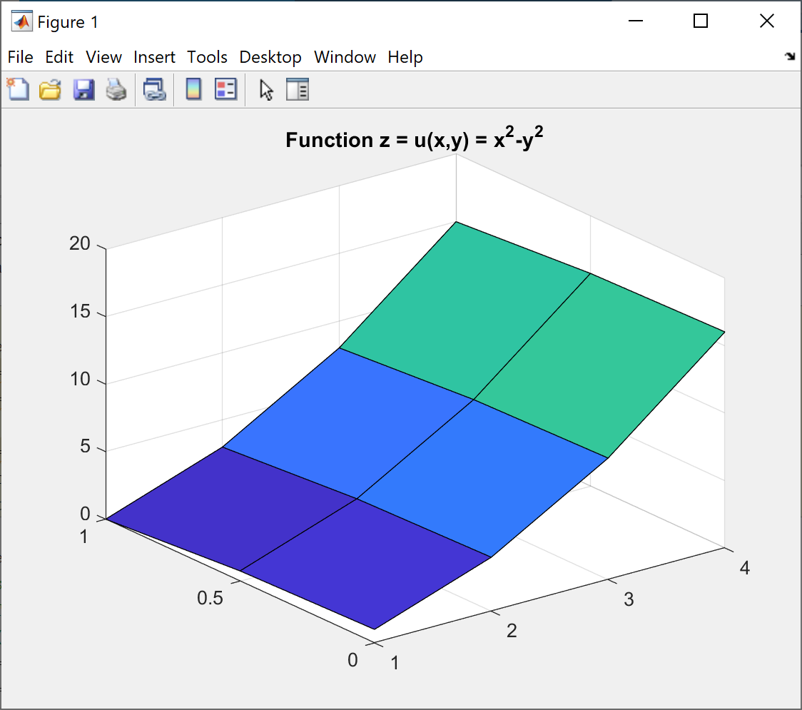
In this example, we create a surface plot of z = u(x, y) = x^2 - y^2 for x- and y-coordinates given as vectors.
- Line 1-2: Create coordinate vectors x and y.
- Line 1-2: Coordinate vectors x and y are used as input to create the matrices X and Y with meshgrid().
- Line 4: Calculate 3x4 matrix Z containing the function values.
- Line 5: Plot surface using surf.
Example: Surface plot
Plot function u(x, y) = x^2 - y^2
x = [1, 2, 3, 4];y = [0, 0.5, 1];[X,Y] = meshgrid(x,y)Z = X.^2 - Y.^2surf(X, Y, Z)
The output in the command window is as shown:
Output X, Y from meshgrid:X =1 2 3 41 2 3 41 2 3 4Y =0 0 0 00.5000 0.5000 0.5000 0.50001.0000 1.0000 1.0000 1.0000Function values Z:Z =1.0000 4.0000 9.0000 16.00000.7500 3.7500 8.7500 15.75000 3.0000 8.0000 15.0000
Figure: Surface plot
Plot function u(x, y) = x^2 - y^2
Example 2: 3D-Plot with surf
We plot the same function u(x,y) = x^2-y^2 over a rectangular area [a, b] x [c, d] and enhance the plot with details: title, axis labels, colorbar. We also show the contours and gradient vector field using the functions contour and quiver. The gradient of a function u(x,y) at a point is the directional derivative of the function; the gradient at all points of the domain defines a vector field that can be plotted using the quiver-function.
- Line 1: Define u as anonymous function.
- Line 2-3: Define rectangle [a, b] x [c, d] and number of data points nx= 10 and ny = 20 for the discretization.
- Line 4: Create evenly spaced x and y-coordinate vectors.
- Line 5: Generate the grid matrices X, Y from the evenly space x- and y-coordinates.
- Line 6: Calculate matrix Z containing the function values.
- Line 7: Calculate the gradient [px, py] of the function
- Line 9-13: Create surface plot of the function u.
- Line 14-20:Create 2D-plot of function with contour lines and gradient vector field.
Example: Surface plot with contour and gradient
Plot function u(x, y) = x^2 - y^2, its contour and gradient
Used functions: surf, contour, quiver
u = @(x,y) x.^2 - y.^2;a = -5; b = 5; nx = 10;c = -10; d = 10; ny = 20;x = linspace(a,b,nx+1);y = linspace(c,d,ny+1);[X,Y] = meshgrid(x,y);Z = u(X,Y);[px,py] = gradient(Z);figure('Position', [50,50,700,500]);subplot(2,1,1)surf(X, Y, Z);xlim([a,b]);ylim([c,d]);view(3);title('Function z = u(x,y) = x^2-y^2')xlabel('x');ylabel('y');zlabel('z = u(x,y)');subplot(2,1,2)contour(X,Y,Z);hold onquiver(X, Y, px, py);title('Contour and gradient')xlabel('x');ylabel('y');xlim([a,b]);ylim([c,d]);colorbar;colormap('jet')
Figure: Surface plot with contour and gradient
Plot function u(x, y) = x^2 - y^2, its contour and gradient
9-6 Advanced plotting
| Top |
This section shows some advanced plotting that can be used in the context of solving ordinary differential equations (ODEs). Firstly, we analyze the qualitative behaviour of the solutions of a population growth model by visualizing them.
Visualize solutions of a population growth model
The population growth y(t) of an organism is modeled using the logistic equation
ODE: y' = c*y - c/k*y^2
IC: y(0) = y0
where c > 0 is the growth rate of the population and k > 0 is the carrying capacity,
that is, the maximum population that the environment can sustain.
In our specific example we set the parameters to c = 1.3 and k = 40.
This ordinary differential equation is solved numerically for a set of initial conditions using MATLAB's ode45 solver.
Example: Visualize solutions of an ODE
We write a loop, in which the ODE is solved for the initial conditions IC = [4, 8, 50, 60] and the solutions y are plotted on the same figure by using the hold on command. Each plot gets its own marker, selected from an array of markers, and its own DisplayName-property, that will be included in the legend. The handle h(i) of each plot is saved in an array h. The legend then can be constructed after the loop using the command legend(h).
% Solve y' = c*y - c/k*y^2 with different IC% Specify the modelc = 1.3; % growth factork = 40; % carrying capacityf = @(t, y) c*y - c/k*y.^2;tspan = [0 10];figuremarkers = {'+','o','*','x'};h = zeros(1,4);i = 1;% Solve the problem using ode45% for different initial conditionsfor IC = [4, 8, 50, 60][t, y] = ode45(f, tspan, IC);h(i) = plot(t, y, 'LineWidth', 1.5, ...'Marker', markers(i), ...'DisplayName', num2str(IC,'y0=%d'));i = i+1;hold onendhold offtitle('Solve dy/dt = c*y - c/k*y^2, c = 2, k = 20');subtitle('Equilibrium at y(t) = 40')legend(h);grid on;xlabel('t'), ylabel('y');
Figure: Visualize solutions of an ODE
The visualization confirms that all solutions approach the equilibrium state at the carrying capacity y(t) = 40. For initial conditions less than k = 40, the population increases towards the equilibrium. For initial conditions greater than k = 40, the population decreases towards the equilibrium.
Functions for plotting: plot, title, subtitle, legend, xlabel, ylabel
Functions for solving ODEs: ode45
10 Symbolic computations
| Top |
The Symbolic Math Toolbox is used to analyze and solve mathematical problems analytically, for example to calculate derivatives,
partial derivatives and integrals of function expressions, to solve equations,
or to plot functions.
The symbolic mode is started by typing the keyword syms followed by the name of the symbolic variables, for example:
syms x
syms x y
syms x y z
Symbolic computations can be done interactively in the command window or in a script. Derivative, integral and gradient of functions are calculated symbolically using the functions diff, int and gradient. For symbolic plots there are a number of functions such as fplot, fsurf and fcontour, their name starts with "f" and they all work on symbolic function expressions.
Code: Symbolic computation
Calculate derivative and integral of functions
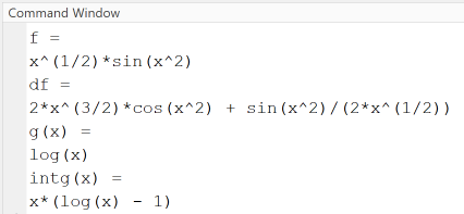
The following example shows how to declare functions of one variable and calculate the derivative using diff and integral using int. Note that the symbolic mode is started in line 1 with the syms keyword and the name of the variable x, and then in line 7 with the syms keyword and the name of the function g(x).
syms x% Declare symbolic function f depending on xf = sin(x^2)*sqrt(x)% Determine derivative of f using diffdf = diff(f)% Declare symbolic function g depending on xsyms g(x)g(x) = log(x)% Determine integral of the function gintg = int(g)% Plot gfplot(g); title("g(x) = log(x)");
Output
Result of symbolic computation
The usage of symbolic computations is helpful when you develop a new numerical method and need to cross-check the numerical solutions with the exact analytical solutions.
If you mix symbolic and numerical computations in a MATLAB script, it is useful to know that symbolic functions can be transformed to function handles using matlabFunction. In the following example we calculate the symbolic exact derivative of a function and then transform it to an anonymous function, so that we can use it for further numerical computations.
syms x% Declare symbolic function f depending on xf = sin(2*x)*exp(2*x)% Determine symbolic derivative of f using diffdf = diff(f) % this df is a symbolic function% Create anonymous function for derivativedf = matlabFunction(df) % now df is a function handle
MATLAB Quizzes
| Top |
Further learning materials include a YouTube Video and two MATLAB Quizzes. The YouTube-Video gives additional insight in how to learn MATLAB basic commands using this tutorial in a step-by-step way.
Test your basic understanding of MATLAB Development Environment and language syntax by taking the MATLAB Quizzes . Each quiz consists of ten questions, each with three to four possible answers, and there may be multiple correct or incorrect answers. Check those answers that you think are correct. If you have answered at least 50% of the answers correctly, you are prepared to take MATLAB a step further, for example by taking the course "Numerical Methods". Have fun!
Tools & References
| Top |
This tutorial gives an introduction to MATLAB basic syntax. Starting here, there is much more to be learned and done. Further interesting topics are: write MATLAB LiveScripts, use the GUI Editor to create graphical user interfaces, write larger programs using classes and inheritance, develop your own toolbox.
- MATLAB Help: https://de.mathworks.com/help/matlab/
- MATLAB Language Fundamentals: https://de.mathworks.com/help/matlab/language-fundamentals.html
- Octave Software: https://www.gnu.org/software/octave/
- This Tutorial as PDF-File: MATLAB Tutorial - First steps in MATLAB _ Prof. E. Kiss, HS KL.pdf
- This Tutorial in German: MATLAB Tutorial - Der Einstieg für Anfänger